 Click or Tap the Example circuits below to invoke TINACloud and select the Interactive DC mode to Analyze them Online.
 Get a low cost access to TINACloud to edit the examples or create your own circuits
There are several different definitions of power in AC circuits; all, however, have dimension of V*A or W (watts).
1. Instantaneous power: p(t) is the time function of the power, p(t) = u(t)*i(t). It is the product of the time functions of the voltage and current. This definition of instantaneous power is valid for signals of any waveform. The unit for instantaneous power is VA.
2. Complex power: S
Complex power is the product of the complex effective voltage and the complex effective conjugate current. In our notation here, the conjugate is indicated by an asterisk (*).Complex power can also be computed using the peak values of the complex voltage and current, but then the result must be divided by 2. Note that complex power is applicable only to circuits with sinusoidal excitation because complex effective or peak values exist and are defined only for sinusoidal signals. The unit for complex power is VA.
3. Real or average power: P can be defined in two ways: as the real part of the complex power or as the simple average of the instantaneous power. The second definition is more general because with it we can define the instantaneous power for any signal waveform, not just for sinusoids. It is given explicitly in the following expression
The unit for real or average power is watts (W), just as for power in DC circuits. Real power is dissipated as heat in resistances.
4. Reactive power: Q is the imaginary part of the complex power. It is given in units of volt-amperes reactive (VAR). Reactive power is positive in an inductive circuit and negative in a capacitive circuit. This power is defined only for sinusoidal excitation. The reactive power doesn’t do any useful work or heat and it is the power returned to the source by the reactive components (inductors, capacitors) of the circuit
5. Apparent power: S is the product of the rms values of the voltage and the current, S = U*I. The unit of apparent power is VA. The apparent power is the absolute value of the complex power, so it is defined only for sinusoidal excitation.
Power Factor (cos φ)
The power factor is very important in power systems because it indicates how closely the effective power equals the apparent power. Power factors near one are desirable. The definition:

TINAӳ power-measuring instrument also measures the power factor.
In our first example, we calculate the powers in a simple circuit.
Example 1
Find the average (dissipated) and reactive powers of the resistor and the capacitor.
Find the average and reactive powers provided by the source.
Check to see if the powers provided by the source equal those in the components.
First calculate the network current.
 = 3.9 ej38.7BмmA
PR= I2*R = (3.052+2.442)*2/2 = 15.2 mW
QC = -I2/wC = -15.2/1.256 = -12.1mVAR

Where you see division by 2, remember that where the peak value is used for the source voltage and the power definition, the power calculation requires the rms value.
Checking the results, you can see that the sum of all three powers is zero, confirming that the power from the source appears at the two components.
The instantaneous power of the voltage source:
pV(t) = -vS(t)*i(t) = -10 cos ωt * 3.9 cos( ω t+38.7 м) = -39cos ω t*( cos ω t cos 38.7 м-sin ω t sin 38.7 м ) = -30.45 cos ω t + 24.4 sin ω tVA
Next, we demonstrate how easy it is to obtain these results using a schematic and instruments in TINA. Note that in the TINA schematics we use TINAӳ jumpers to connect the power meters.
You can obtain the above tables by selecting Analysis/AC Analysis/Calculate nodal voltages from the menu and then clicking the power meters with the probe.
We can conveniently determine the apparent power of the voltage source using TINAӳ Interpreter:
 S = VS*I = 10*3.9/2 = 19.5 VA
om:=2*pi*1000;
V:=10;
I:=V/(R+1/(j*om*C));
Iaq:=sqr(abs(I));
PR:=Iaq*R/2;
PR=[15.3068m]
QC:=Iaq/(om*C*2);
QC=[12.1808m]
Ic:=Re(I)-j*Im(I);
Sv:=-V*Ic/2;
Sv=[-15.3068m+12.1808m*j]
import math as m
import cmath as c
#Lets simplify the print of complex
#numbers for greater transparency:
cp= lambda Z : “{:.4f}”.format(Z)
om=2000*c.pi
V=10
I=V/(R+1/1j/om/C)
laq=abs(I)**2
PR=laq*R/2
print(“PR=”,cp(PR))
QC=laq/om/C/2
print(“QC=”,cp(QC))
Ic=I.conjugate()
Sv=-V*Ic/2
print(“Sv=”,cp(Sv))
You can see that there are ways other than the definitions themselves to calculate the power in two-pole networks. The following table summarizes this:
| P | Q |  | S | |
|---|---|---|---|---|
| Z = R + jX | R*I2 | X*I2 | ½Z½*I2 | Z*I2 |
| Y = G + jB | G*V2 | -B*V2 | ½Y½*V2 |  V2 V2 |
In this table, we have rows for circuits characterized by either their impedance or their admittance. Be careful using the formulas. When considering the impedance form, think of the impedance as representing a series circuit, for which you need the current. When considering the admittance form, think of the admittance as representing a parallel circuit, for which you need the voltage. And donӴ forget that although Y = 1/Z, in general G ≠ 1/R. Except for the special case X = 0 (pure resistance), G = R/( R2+ X2 ).
Example 2
Find the average power, the reactive power, p(t), and the power factor of the two-pole network connected to the current source.
iS(t)=(100 * cos ω t)mA w = 1 krad/s
Refer to the table above and, since the two-pole network is a parallel circuit, use the equations in the row for the admittance case.
Working with an admittance, we must first find the admittance itself. Fortunately, our two-pole network is a purely parallel one.
Yeq= 1/R + j ω C + 1/j ω L = 1/5 + j250*10-6103 + 1/(j*20*10-3103) = 0.2+j0.2 S
We need the absolute value of the voltage:
½V ½= ½Z ½*I= I/ ½Y ½= 0.1/ ê(0.2+j0.2) ê=0.3535 V
The powers:
P = V2*G = 0.125*0.2/2 = 0.0125 W
Q = -V2*B = – 0.125*0.2/2 = – 0.0125 var
 = V2*
= V2* =0.125* (0.2-j0.2)/2 = ( 12.5 – j 12.5 ) mVA
S = V2* Y = 0.125* ê0.2+j0.2 ê/2 = 0.01768 VA
cos φ = P/S = 0.707
om:=1000;
Is:=0.1;
V:=Is*(1/(1/R+j*om*C+1/(j*om*L)));
V=[250m-250m*j]
S:=V*Is/2;
S=[12.5m-12.5m*j]
P:=Re(S);
Q:=Im(S);
P=[12.5m]
Q=[-12.5m]
abs(S)=[17.6777m]
#Lets simplify the print of complex
#numbers for greater transparency:
cp= lambda Z : “{:.4f}”.format(Z)
om=1000
Is=0.1
V=Is*(1/(1/R+1j*om*C+1/1j/om/L))
print(“V=”,cp(V))
S=V*Is/2
P=S.real
Q=S.imag
print(“P=”,cp(P))
print(“Q=”,cp(Q))
print(“abs(S)=”,cp(abs(S)))
Example 3
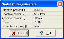
Find the average and reactive powers of the two-pole network connected to the voltage generator.
For this example, we will dispense with manual solutions and show how to use TINAӳ measuring instruments and Interpreter to obtain the answers.
Selec Analysis/AC Analysis/Calculate nodal voltages from the menu and then click the power meter with the probe. The following table will appear:
Vs:=100;
om:=1E8*2*pi;
Ie:=Vs/(R2+1/j/om/C2+replus(replus(R1,j*om*L),1/j/om/C1));
Ze:=(R2+1/j/om/C2+replus(replus(R1,j*om*L),1/j/om/C1));
P:=sqr(abs(Ie))*Re(Ze)/2;
Q:=sqr(abs(Ie))*Im(Ze)/2;
P=[14.6104]
Q=[-58.7055]
import cmath as c
#Lets simplify the print of complex
#numbers for greater transparency:
cp= lambda Z : “{:.4f}”.format(Z)
#Define replus using lambda:
Replus= lambda R1, R2 : R1*R2/(R1+R2)
Vs=100
om=200000000*c.pi
Ie=Vs/(R2+1/1j/om/C2+Replus(Replus(R1,1j*om*L),1/1j/om/C1))
Ze=R2+1/1j/om/C2+Replus(Replus(R1,1j*om*L),1/1j/om/C1)
p=abs(Ie)**2*Ze.real/2
print(“p=”,cp(p))