 Click or Tap the Example circuits below to invoke TINACloud and select the Interactive DC mode to Analyze them Online.
 Get a low cost access to TINACloud to edit the examples or create your own circuits
We have already shown how the elementary methods of DC circuit analysis can be extended and used in AC circuits to solve for the complex peak or effective values of voltage and current and for complex impedance or admittance. In this chapter, we’ll solve some examples of voltage and current division in AC circuits.
Example 1
Find the voltages v1(t) and v2(t), given that vs(t)=110cos(2p50t).
Let’s first obtain this result by hand calculation using the voltage division formula.
The problem can be considered as two complex impedances in series: the impedance of the resistor R1, Z1=R1 ohms (which is a real number), and the equivalent impedance of R2 and L2 in series, Z2 = R2 + j w L2.
Substituting the equivalent impedances, the circuit can be redrawn in TINA as follows:
Note that we have used a new component, a complex impedance, now available in TINA v6. You can define the frequency dependence of Z by means of a table that you can reach by double clicking the impedance component. In the first row of the table you can define either the DC impedance or a frequency independent complex impedance (we have done the latter here, for the inductor and resistor in series, at the given frequency).
Using the formula for voltage division:
V1 = Vs*Z1 / (Z1 + Z2)
V2 = Vs*Z2 / (Z1 + Z2)
Numerically:
Z1 = R1 = 10 ohms
Z2 = R2 + j w L = 15 + j 2*p* 50*0.04 =15 + j 12.56 ohms
V1= 110*10/ (25+j12.56) = 35.13-j17.65 V = 39.31 e –j26.7 ° V
V2= 110*(15+j12.56)/ (25+j12.56) = 74.86+j17.65 V = 76.92 e j 13.3° V
The time function of the voltages:
v1(t) = 39.31 cos (wt – 26.7°) V
v2(t) = 76.9 cos (wt + 13.3°) V
Let’s check the result with TINA using Analysis/AC Analysis/Calculate nodal voltagesV1
V2
Next let’s check these results with TINA’s Interpreter:
f:=50;
om:=2*pi*f;
VS:=110;
v1:=VS*R1/(R1+R2+j*om*L2);
v2:=VS*(R2+j*om*L2)/(R1+R2+j*om*L2);
v1=[35.1252-17.6559*j]
v2=[74.8748+17.6559*j]
abs(v2)=[76.9283]
radtodeg(arc(v2))=[13.2683]
abs(v1)=[39.313]
radtodeg(arc(v1))=[-26.6866]
import math as m
import cmath as c
#Lets simplify the print of complex
#numbers for greater transparency:
cp= lambda Z : “{:.4f}”.format(Z)
f=50
om=2*c.pi*f
VS=110
v1=VS*R1/complex(R1+R2,om*L2)
v2=VS*complex(R2,om*L2)/complex(R1+R2,om*L2)
print(“v1=”,cp(v1))
print(“v2=”,cp(v2))
print(“abs(v1)= %.4f”%abs(v1))
print(“degrees(arc(v1))= %.4f”%m.degrees(c.phase(v1)))
print(“abs(v2)= %.4f”%abs(v2))
print(“arc(v2)*180/pi= %.4f”%(c.phase(v2)*180/c.pi))
Note that when using the Interpreter we did not have to declare the values of the passive components. This is because we are using the Interpreter in a work session with TINA in which the schematic is in the schematic editor. TINA’s Interpreter looks in this schematic for the definition of the passive component symbols entered into the Interpreter program.
Finally, let’s use TINA’s Phasor Diagram to demonstrate this result. Connecting a voltmeter to the voltage generator, selecting the Analysis/AC Analysis/Phasor Diagram command, setting the axes, and adding the labels, will yield the following diagram. Note that View/Vector label style was set to Amplitude for this diagram.
The diagram shows that Vs is the sum of the phasors V1 and V2, Vs = V1 + V2.
By moving the phasors we can also demonstrate that V2 is the difference between Vs and V1, V2 = Vs – V1.
This figure also demonstrates the subtraction of vectors. The resultant vector should start from the tip of the second vector, V1.
In a similar way we can demonstrate that V1 = Vs – V2. Again, the resultant vector should start from the tip of the second vector, V1.
Of course, both phasor diagrams can be considered as a simple triangle rule diagram for Vs = V1 + V2 .
The phasor diagrams above also demonstrate Kirchhoff’s voltage law (KVL).
As we have learned in our study of DC circuits, the applied voltage of a series circuit equals the sum of the voltage drops across the series elements. The phasor diagrams demonstrate that KVL is also true for AC circuits, but only if we use complex phasors!
Example 2
In this circuit, R1 represents the DC resistance of the coil L; together they model a real world inductor with its loss component. Find the voltage across the capacitor and the voltage across the real world coil.
L = 1.32 h, R1 = 2 kohms, R2 = 4 kohms, C = 0.1 mF, vS(t) = 20 cos (wt) V, f = 300Hz.
 V2
V2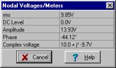
Solving by hand using voltage division:
= 13.91 e j 44.1° V
and
v1(t) = 13.9 cos (w×t + 44°) V
= 13.93 e –j 44.1° V
and
v2(t) = 13.9 cos(w×t – 44.1°) V
Notice that at this frequency, with these component values, the magnitudes of the two voltages are nearly the same, but the phases are of opposite sign.
Once again, let’s have TINA do the tedious work by solving for V1 and V2 with the Interpreter:
om:=600*pi;
V:=20;
v1:=V*(R1+j*om*L)/(R1+j*om*L+replus(R2,(1/j/om/C)));
abs(v1)=[13.9301]
180*arc(v1)/pi=[44.1229]
v2:=V*(replus(R2,1/j/om/C))/(R1+j*om*L+replus(R2,(1/j/om/C)));
abs (v2)=[13.9305]
180*arc(v2)/pi=[-44.1211]
import math as m
import cmath as c
#Lets simplify the print of complex
#numbers for greater transparency:
cp= lambda Z : “{:.4f}”.format(Z)
#Define replus using lambda:
Replus= lambda R1, R2 : R1*R2/(R1+R2)
om=600*c.pi
V=20
v1=V*complex(R1,om*L)/complex(R1+1j*om*L+Replus(R2,1/1j/om/C))
print(“abs(v1)= %.4f”%abs(v1))
print(“180*arc(v1)/pi= %.4f”%(180*c.phase(v1)/c.pi))
v2=V*complex(Replus(R2,1/1j/om/C))/complex(R1+1j*om*L+Replus(R2,1/1j/om/C))
print(“abs(v2)= %.4f”%abs(v2))
print(“180*arc(v2)/pi= %.4f”%(180*c.phase(v2)/c.pi))
And finally, take a look at this result using TINA’s Phasor Diagram. Connecting a voltmeter to the voltage generator, invoking the Analysis/AC Analysis/Phasor Diagram command, setting the axes, and adding the labels will yield the following diagram (note that we have set View/Vector label style to Real+j*Imag for this diagram):
Example 3
The current source iS(t) = 5 cos (wt) A, the resistor R = 250 mohm, the inductor L = 53 uH, and the frequency f = 1 kHz. Find the current in the inductor and the current in the resistor. 
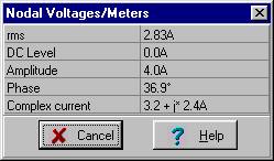
Using the formula for current division:

iR(t) = 4 cos (w×t + 37.2°) A
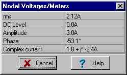
Similarly:


iL(t) = 3 cos(w×t – 53.1°)
And using the Interpreter in TINA:
om:=2*pi*1000;
is:=5;
iL:=is*R/(R+j*om*L);
iL=[1.8022-2.4007*j]
iR:=is*j*om*L/(R+j*om*L);
iR=[3.1978+2.4007*j]
abs(iL)=[3.0019]
radtodeg(arc(iL))=[-53.1033]
abs(iR)=[3.9986]
radtodeg(arc(iR))=[36.8967]
import math as m
import cmath as c
#Lets simplify the print of complex
#numbers for greater transparency:
cp= lambda Z : “{:.4f}”.format(Z)
om=2*c.pi*1000
i=5
iL=i*R/complex(R+1j*om*L)
print(“iL=”,cp(iL))
iR=complex(i*1j*om*L/(R+1j*om*L))
print(“iR=”,cp(iR))
print(“abs(iL)= %.4f”%abs(iL))
print(“degrees(arc(iL))= %.4f”%m.degrees(c.phase(iL)))
print(“abs(iR)= %.4f”%abs(iR))
print(“degrees(arc(iR))= %.4f”%m.degrees(c.phase(iR)))
We can also demonstrate this solution with a phasor diagram:
The phasor diagram shows that the generator current IS is the resultant vector of the complex currents IL and IR. It also demonstrates Kirchhoff’s current law (KCL), showing that the current IS entering the upper node of the circuit equals the sum of IL and IR, the complex currents leaving the node.
Example 4
Determine i0(t), i1(t) and i2(t). The component values and the source voltage, frequency, and phase are given on the schematic below.
i0

i1
i2

In our solution, we will use the principle of current division. First we find the expression for the total current i0:
I0M = 0.315 e j 83.2° A and i0(t) = 0.315 cos (w×t + 83.2°) A
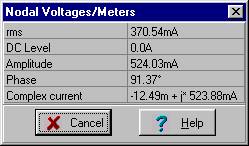
Then using current division, we find the current in the capacitor C:
I1M = 0.524 e j 91.4° A and i1(t) = 0.524 cos(w×t + 91.4°) A
And the current in the inductor:
I2M = 0.216 e–j 76.6° A and i2(t) = 0.216 cos(w×t – 76.6°) A
With anticipation, we seek confirmation of our hand calculations using TINA’s Interpreter.
V:=10;
om:=2*pi*1000;
I0:=V/((1/j/om/C1)+replus((1/j/om/C),(R+j*om*L)));
I0=[37.4671m+313.3141m*j]
abs(I0)=[315.5463m]
180*arc(I0)/pi=[83.1808]
I1:=I0*(R+j*om*L)/(R+j*om*L+1/j/om/C);
I1=[-12.489m+523.8805m*j]
abs(I1)=[524.0294m]
180*arc(I1)/pi=[91.3656]
I2:=I0*(1/j/om/C)/(R+j*om*L+1/j/om/C);
I2=[49.9561m-210.5665m*j]
abs(I2)=[216.4113m]
180*arc(I2)/pi=[-76.6535]
{Control: I1+I2=I0}
abs(I1+I2)=[315.5463m]
import math as m
import cmath as c
#Lets simplify the print of complex
#numbers for greater transparency:
cp= lambda Z : “{:.4f}”.format(Z)
#First define replus using lambda:
Replus= lambda R1, R2 : R1*R2/(R1+R2)
V=10
om=2*c.pi*1000
I0=V/complex((1/1j/om/C1)+Replus(1/1j/om/C,R+1j*om*L))
print(“I0=”,cp(I0))
print(“abs(I0)= %.4f”%abs(I0))
print(“180*arc(I0)/pi= %.4f”%(180*c.phase(I0)/c.pi))
I1=I0*complex(R,om*L)/complex(R+1j*om*L+1/1j/om/C)
print(“I1=”,cp(I1))
print(“abs(I1)= %.4f”%abs(I1))
print(“180*arc(I1)/pi= %.4f”%(180*c.phase(I1)/c.pi))
I2=I0*complex(1/1j/om/C)/complex(R+1j*om*L+1/1j/om/C)
print(“I2=”,cp(I2))
print(“abs(I2)= %.4f”%abs(I2))
print(“180*arc(I2)/pi= %.4f”%(180*c.phase(I2)/c.pi))
#Controll: I1+I2=I0
print(“abs(I1+I2)= %.4f”%abs(I1+I2))
Another way of solving this would be to first find the voltage across the parallel complex impedance of ZLR and ZC. Knowing this voltage, we could find the currents i1 and i2 by then dividing this voltage first by ZLR and then by ZC. We will show next the solution for voltage across the parallel complex impedance of ZLR and ZC. We will have to use the voltage division principal along the way:
VRLCM = 8.34 e j 1.42° V
and
IC = I1= VRLCM*jwC = 0.524 e j 91.42° A
and hence
iC (t) = 0.524 cos (w×t + 91.4°) A.