Click or Tap the Example circuits below to invoke TINACloud and select the Interactive DC mode to Analyze them Online.
 Get a low cost access to TINACloud to edit the examples or create your own circuits
As we have already seen, circuits with sinusoidal excitation can be solved using complex impedances for the elements and complex peak or complex rms values for the currents and voltages. Using the complex values version of Kirchhoff’s laws, nodal and mesh analysis techniques can be employed to solve AC circuits in a manner similar to DC circuits. In this chapter we will show this through examples of Kirchhoff’s laws.
Example 1
Find the amplitude and phase angle of the current ivs(t) if
vS(t) = VSM cos 2pft; i(t) =ISM cos 2pft; VSM = 10 V; ISM = 1 A; f = 10 kHz;
Altogether we have 10 unknown voltages and currents, namely: i, iC1, iR, iL, iC2, vC1, vR, vL, vC2 and vIS. (If we use complex peak or rms values for the voltages and currents, we have altogether 20 real equations!)
The equations:
Loop or mesh equations: for M1 – VSM +VC1M+VRM = 0
M2 – VRM + VLM = 0
M3 – VLM + VC2M = 0
M4 – VC2M + VIsM = 0
Ohm’s laws VRM = R*IRM
VLM = j*w*L*ILM
IC1M = j*w*C1*VC1M
IC2M = j*w*C2*VC2M
Nodal equation for N1 – IC1M – ISM + IRM + ILM +IC2M = 0
for series elements I = IC1MSolving the system of equations you can find the unknown current:
ivs (t) = 1.81 cos (wt + 79.96°) A
Solving such a large system of complex equations is very complicated, so we haven’t shown it in detail. Each complex equation leads to two real equations, so we show the solution only by the values calculated with TINA’s Interpreter.
The solution using TINA’s Interpreter:
om:=20000*pi;
Vs:=10;
Is:=1;
Sys Ic1,Ir,IL,Ic2,Vc1,Vr,VL,Vc2,Vis,Ivs
Vs=Vc1+Vr {M1}
Vr=VL {M2}
Vr=Vc2 {M3}
Vc2=Vis {M4}
Ivs=Ir+IL+Ic2-Is {N1}
{Ohm’s rules}
Ic1=j*om*C1*Vc1
Vr=R*Ir
VL=j*om*L*IL
Ic2=j*om*C2*Vc2
Ivs=Ic1
end;
Ivs=[3.1531E-1+1.7812E0*j]
abs(Ivs)=[1.8089]
fiIvs:=180*arc(Ivs)/pi
fiIvs=[79.9613]
import sympy as s
import cmath as c
cp= lambda Z : “{:.4f}”.format(Z)
om=20000*c.pi
Vs=10
Is=1
Ic1,Ir,IL,Ic2,Vc1,Vr,VL,Vc2,Vis,Ivs=s.symbols(‘Ic1 Ir IL Ic2 Vc1 Vr VL Vc2 Vis Ivs’)
A=[s.Eq(Vc1+Vr,Vs),s.Eq(VL,Vr),s.Eq(Vc2,Vr),s.Eq(Vis,Vc2), #M1, M2, M3, M4
s.Eq(Ir+IL+Ic2-Is,Ivs), #N1
s.Eq(1j*om*C1*Vc1,Ic1),s.Eq(R*Ir,Vr),s.Eq(1j*om*L*IL,VL),s.Eq(1j*om*C2*Vc2,Ic2),s.Eq(Ic1,Ivs)] #Ohm’s rules
Ic1,Ir,IL,Ic2,Vc1,Vr,VL,Vc2,Vis,Ivs=[complex(Z) for Z in tuple(s.linsolve(A,(Ic1,Ir,IL,Ic2,Vc1,Vr,VL,Vc2,Vis,Ivs)))[0]]
print(Ivs)
print(“abs(Ivs)=”,cp(abs(Ivs)))
print(“180*c.phase(Ivs)/c.pi=”,cp(180*c.phase(Ivs)/c.pi))
The solution using TINA:
To solve this problem by hand, work with the complex impedances. For example, R, L and C2 are connected in parallel, so you can simplify the circuit by computing their parallel equivalent. || means the parallel equivalent of the impedances:
Numerically:

The simplified circuit using the impedance:
The equations in ordered form : I + IG1 = IZ
VS = VC1 +VZ
VZ = Z · IZ
I = j w C1· VC1
There are four unknowns- I; IZ; VC1; VZ – and we have four equations, so a solution is possible.
Express I after substituting the other unknowns from the equations:

Numerically
According to TINA’s Interpreter’s result.
om:=20000*pi;
Vs:=10;
Is:=1;
Z:=replus(R,replus(j*om*L,1/j/om/C2));
Z=[2.1046E0-2.4685E0*j]
sys I
I=j*om*C1*(Vs-Z*(I+Is))
end;
I=[3.1531E-1+1.7812E0*j]
abs(I)=[1.8089]
180*arc(I)/pi=[79.9613]
import sympy as s
import cmath as c
Replus= lambda R1, R2 : R1*R2/(R1+R2)
om=20000*c.pi
Vs=10
Is=1
Z=Replus(R,Replus(1j*om*L,1/1j/om/C2))
print(‘Z=’,cp(Z))
I=s.symbols(‘I’)
A=[s.Eq(1j*om*C1*(Vs-Z*(I+Is)),I),]
I=[complex(Z) for Z in tuple(s.linsolve(A,I))[0]][0]
print(“I=”,cp(I))
print(“abs(I)=”,cp(abs(I)))
print(“180*c.phase(I)/c.pi=”,cp(180*c.phase(I)/c.pi))
The time function of the current, then, is:
i(t) = 1.81 cos (wt + 80°) A
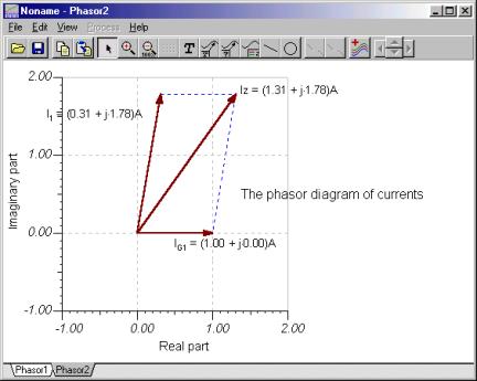
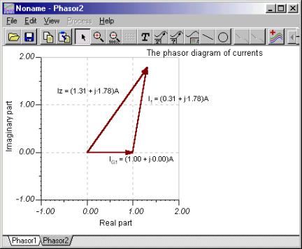
You can check Kirchhoff’s current rule using phasor diagrams. The picture below was developed by checking the node equation in iZ = i + iG1 form. The first diagram shows the phasors added by parallelogram rule, the second one illustrates the triangular rule of the phasor addition.
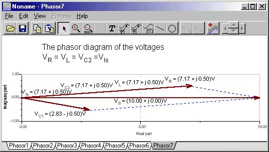
Now let’s demonstrate KVR using TINA’s phasor diagram feature. Since the source voltage is negative in the equation, we connected the voltmeter “backwards.” The phasor diagram illustrates the original form of the Kirchhoff’s voltage rule.
The first phasor diagram uses the parallelogram rule, while the second uses the triangular rule.
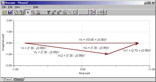
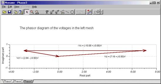
To illustrate KVR in the form VC1 + VZ – VS = 0, we again connected the voltmeter to the voltage source backwards. You can see that the phasor triangle is closed.
Example 2
Find the voltages and currents of all the components if:
vS(t) = 10 cos wt V, iS(t) = 5 cos (w t + 30°) mA;
C1 = 100 nF, C2 = 50 nF, R1 = R2 = 4 k; L = 0.2 H, f = 10 kHz.
Let the unknowns be the complex peak values of the voltages and currents of ‘passive’ elements, as well as the current of the voltage source ( iVS ) and the voltage of the current source ( vIS ). Altogether, there are twelve complex unknowns. We have three independent nodes, four independent loops ( marked as MI), and five passive elements which can be characterized by five “Ohm’s laws” – altogether there are 3+4+5 = 12 equations:
Nodal equations for N1 IVsM = IR1M + IC2M
for N2 IR1M = ILM + IC1M
for N3 IC2M + ILM + IC1M +IsM = IR2M
Loop equations for M1 VSM = VC2M + VR2M
for M2 VSM = VC1M + VR1M+ VR2M
for M3 VLM = VC1M
for M4 VR2M = VIsM
Ohm’s laws VR1M = R1*IR1M
VR2M = R2*IR2M
IC1m = j*w*C1*VC1M
IC2m = j*w*C2*VC2M
VLM = j*w*L*ILM
Don’t forget that any complex equation might lead to two real equations, so Kirchhoff’s method requires many calculations. It’s much simpler to solve for the time functions of the voltages and currents using a system of differential equations (not discussed here). First we show the results calculated by TINA’s Interpreter:
f:=10000;
Vs:=10;
s:=0.005*exp(j*pi/6);
om:=2*pi*f;
sys ir1, ir2, ic1, ic2, iL, vr1, vr2, vc1, vc2, vL, vis, ivs
ivs=ir1+ic2 {1}
ir1=iL+ic1 {2}
ic2+iL+ic1+Is=ir2 {3}
Vs=vc2+vr2 {4}
Vs=vr1+vr2+vc1 {5}
vc1=vL {6}
vr2=vis {7}
vr1=ir1*R1 {8}
vr2=ir2*R2 {9}
ic1=j*om*C1*vc1 {10}
ic2=j*om*C2*vc2 {11}
vL=j*om*L*iL {12}
end;
abs(vr1)=[970.1563m]
abs(vr2)=[10.8726]
abs(ic1)=[245.6503u]
abs(ic2)=[3.0503m]
abs(vc1)=[39.0965m]
abs(vc2)=[970.9437m]
abs(iL)=[3.1112u]
abs(vL)=[39.0965m]
abs(ivs)=[3.0697m]
180+radtodeg(arc(ivs))=[58.2734]
abs(vis)=[10.8726]
radtodeg(arc(vis))=[-2.3393]
radtodeg(arc(vr1))=[155.1092]
radtodeg(arc(vr2))=[-2.3393]
radtodeg(arc(ic1))=[155.1092]
radtodeg(arc(ic2))=[-117.1985]
radtodeg(arc(vc2))=[152.8015]
radtodeg(arc(vc1))=[65.1092]
radtodeg(arc(iL))=[-24.8908]
radtodeg(arc(vL))=[65.1092]
import sympy as s
import math as m
import cmath as c
cp= lambda Z : “{:.4f}”.format(Z)
f=10000
Vs=10
S=0.005*c.exp(1j*c.pi/6)
om=2*c.pi*f
ir1,ir2,ic1,ic2,iL,vr1,vr2,vc1,vc2,vL,vis,ivs=s.symbols(‘ir1 ir2 ic1 ic2 iL vr1 vr2 vc1 vc2 vL vis ivs’)
A=[s.Eq(ir1+ic2,ivs), #1
s.Eq(iL+ic1,ir1), #2
s.Eq(ic2+iL+ic1+Is,ir2), #3
s.Eq(vc2+vr2,Vs), #4
s.Eq(vr1+vr2+vc1,Vs), #5
s.Eq(vL,vc1), #6
s.Eq(vis,vr2), #7
s.Eq(ir1*R1,vr1), #8
s.Eq(ir2*R2,vr2), #9
s.Eq(1j*om*C1*vc1,ic1), #10
s.Eq(1j*om*C2*vc2,ic2), #11
s.Eq(1j*om*L*iL,vL)] #12
ir1,ir2,ic1,ic2,iL,vr1,vr2,vc1,vc2,vL,vis,ivs=[complex(Z) for Z in tuple(s.linsolve(A,(ir1,ir2,ic1,ic2,iL,vr1,vr2,vc1,vc2,vL,vis,ivs)))[0]]
print(“abs(vr1)=”,cp(abs(vr1)))
print(“abs(vr2)=”,cp(abs(vr2)))
print(“abs(ic1)=”,cp(abs(ic1)))
print(“abs(ic2)=”,cp(abs(ic2)))
print(“abs(vc1)=”,cp(abs(vc1)))
print(“abs(vc2)=”,cp(abs(vc2)))
print(“abs(iL)=”,cp(abs(iL)))
print(“abs(vL)=”,cp(abs(vL)))
print(“abs(ivs)=”,cp(abs(ivs)))
print(“180+degrees(phase(ivs))=”,cp(180+m.degrees(c.phase(ivs))))
print(“abs(vis)=”,cp(abs(vis)))
print(“degrees(phase(vis))=”,cp(m.degrees(c.phase(vis))))
print(“degrees(phase(vr1))=”,cp(m.degrees(c.phase(vr1))))
print(“degrees(phase(vr2))=”,cp(m.degrees(c.phase(vr2))))
print(“degrees(phase(ic1))=”,cp(m.degrees(c.phase(ic1))))
print(“degrees(phase(ic2))=”,cp(m.degrees(c.phase(ic2))))
print(“degrees(phase(vc2))=”,cp(m.degrees(c.phase(vc2))))
print(“degrees(phase(vc1))=”,cp(m.degrees(c.phase(vc1))))
print(“degrees(phase(iL))=”,cp(m.degrees(c.phase(iL))))
print(“degrees(phase(vL))=”,cp(m.degrees(c.phase(vL))))
Now try to simplify the equations by hand using substitution. First substitute eq.9. into eq 5.
VS = VC2 + R2 IR2 a.)
then eq.8 and eq.9. into eq 5.
VS = VC1 + R2 IR2 + R1 IR1 b.)
then eq 12., eq. 10. and IL from eq. 2 into eq.6.
VC1 = VL = jwL IL = jwL(IR1 – IC1) = jwL IR1 – jwL jwC1 VC1
Express VC1
 c.)
c.)
Express VC2 from eq.4. and eq.5. and substitute eq.8., eq.11. and VC1:
 d.)
d.)
Substitute eq.2., 10., 11. and d.) into eq.3. and express IR2
IR2 = IC2 + IR1 + IS = jwC2 VC2 + IR1 + IS
 e.)
e.)
Now substitute d.) and e.) into eq.4 and express IR1
Numerically:
The time function of iR1 is the following:
iR1(t) = 0.242 cos (wt+155.5°) mA
The measured voltages: