In this video we will create and analyze an RLC circuit on the Raspberry Pi 5 single board computer with TINA.
First you have to install the Wine Windows emulator available from the PI-Apps application.
If Wine setup is complete you will see it in the Raspberry OS main menu, so for example you can launch the program WineCfg to configure the optimal text size of the emulated Windows applications.
Assuming you have Wine working in 64-bit mode, you can start the installation of TINA. After completion of the TINA installer, you’ll find TINA in the Raspberry OS main menu (if not in the first level menu, look for it in Wine applications) so you can start it from there.
Creating the RLC circuit
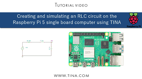
An RLC circuit is an electrical circuit consisting of a Resistor (R), an Inductor (L) and a Capacitor (C). After creating the circuit, we change the default values of some of the components.
Transient Analysis
We Set End display time to 50 microseconds, then select the “Zero initial values”option. Next, we add the diagram to the Schematic Editor window to store it together with the circuit schematic.
Symbolic Analysis
After that, we generate the accurate closed formula describing the transient response using the Symbolic Analysis capability of TINA. Note that the closed formula exists in linear circuits only. The symbolic result describes the transient response of the circuit with an accurate analytic closed formula.
In the following, we will show, how to Draw a diagram using the formula and compare it with the numerical result.
AC Analysis
In the AC Transfer Analysis dialog, set the number of points to 500 to have a finer diagram. Using the checkboxes in the diagram group, you can determine which diagrams will be displayed. Check them all.
The AC Amplitude Characteristic appears, but at the same time the program has calculated the Phase, Nyquist, Group Delay and the AC Bode diagrams.
Symbolic Analysis
Finally, we generate the closed formula of the AC Transfer Function using Symbolic Analysis.
Content of the video:
- 00:00 Introduction
- 02:07 Creating the circuit and changing the default values of some of the components
- 04:21 Transient Analysis
- 05:39 Symbolic Analysis: Semi-symbolic Transient
- 07:47 AC Analysis
- 09:15 Symbolic Analysis: AC Transfer
- 10:25 Conclusion
Click here to watch our video.
You can learn more about TINACloud here: www.tinacloud.com
You can learn more about TINA here: www.tina.com