Month: April 2021

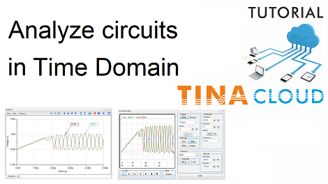
In this tutorial we will demonstrate how to use the virtual oscilloscope in TINACloud.

In practice we very often use an oscilloscope to measure, analyze and debug circuits in the time domain. So, it seems obvious that a simulated oscilloscope can be used in circuit simulation as well. However there are a few important things you must know about.

Even if you analyze the circuits in the computer with a simulated oscilloscope it is still simulation. You should not consider it as measurement, unless you use real time data acquisition for obtaining the data.

The simulated oscilloscope is very useful when you want to adjust some component values of small circuits and want to see the effect of the changes immediately, in order to fine-tune your circuit.

We present the use of the virtual oscillator through an example: Collpitts Oscillator circuit.

• First load the Colpitts.tsc circuit from the TINA Examples folder of TINACloud.
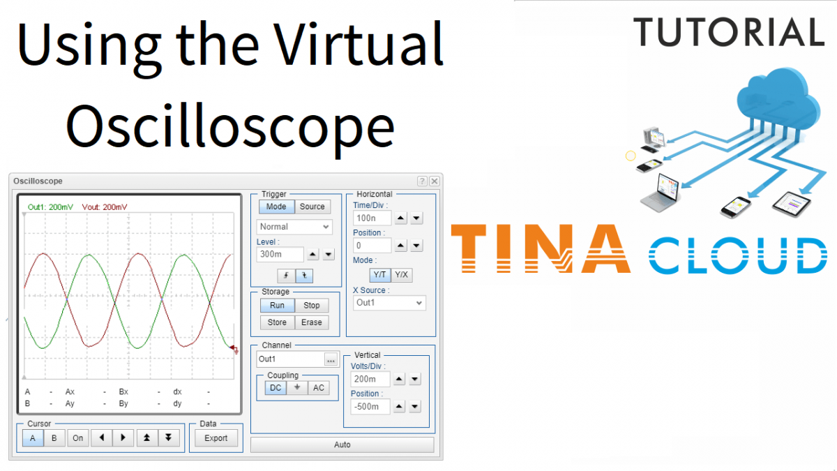
• Next invoke the Oscilloscope from the T&M menu,
• then press the Run button.

As a result , the Out1 signal appears. By default, the oscilloscope is in the “Auto” i. e., free running mode.

To get a steady state image you should enable triggering as follows:

• Set the Trigger Mode to Normal
• next, set Trigger Source to Out1
• finally, set the Trigger Level to 300m.

Consequently, the waveform is stabilized.

With the controls of the Oscilloscope you can make a lot of changes on the displayed waveform.

Here are a few:

By default, on the Oscilloscope rising edge triggering is used, so the display starts when the signal rises above the Trigger level.

• You can also set this to falling edge triggering where the display starts when the signal falls below the Trigger level.

• You can also bring in the Vout signal by selecting Vout under Channel

Let’s have the same vertical settings for Vout as for Out1.

• Finally, you can export the display into a diagram by pressing the Export to Diagram button under Data.

To watch our tutorial and learn more please click  here.

You can learn more about TINA here: www.tina.com

You can learn more about TINACloud here: www.tinacloud.com

In this tutorial video, we will demonstrate and compare the tools available in TINACloud for analyzing circuits in time domain. In TINACloud, you can analyze circuits in time domain, employing two different tools:

• Transient analysis from the Analysis menu of TINACloud.
• Simulated virtual oscilloscope from the T&M menu of TINACloud.

Transient analysis

The Transient analysis calculates the time response of circuits and presents the results as diagrams or text.

Select Transient from the Analysis menu of TINACloud, then press the Run button.

It is also important to select an option related to the Start condition.

For oscillators, like our circuit, the Zero initial values option applies. For amplifiers and many other circuits, you should use the default “Calculate operating point” option. You can refine the diagram in several ways. Here are a few:

• Zoom into any part of the diagram.
• Run cursors on the curves of the diagram.
• Calculate the frequency of the oscillation.
• Mark a period of the signal with the cursors.
• You can also find the Local or Global Minimum or Maximum by clicking the actual value field of a curve.
• You can also enter values to set the cursors more precisely, or
• add Labels to the curves showing the name of the related output on the circuit.
• Separate the curves or collect them in one diagram.
• You can insert the diagram into the schematics and save them together.

Simulated Virtual Oscilloscope

Now, let’s learn to operate the simulated virtual oscilloscope.

The simulated oscilloscope is very useful when you want to adjust some component values of small circuits and want to see the effect of the changes immediately, in order to fine-tune your circuit.

Invoke the oscilloscope from the T&M menu. After pressing the Run button the Out1 signal appears.

Use the controls to make the curve bigger and more detailed.

By default, the oscilloscope is in the “Auto” i. e., free running mode.

To get a steady state image you should enable triggering as follows:

Set the Trigger Mode to Normal

Set Trigger Source to Out1

Set the Trigger Level to 300m.

Consequently, the waveform is stabilized.

With the controls of the oscilloscope you can make a lot of changes on the displayed waveform. Here are a few:

By default, on the oscilloscope rising edge triggering is used, so the display starts when the signal rises above the Trigger level.

• You can also set this to falling edge triggering where the display starts when the signal falls below the Trigger level.
• You can also bring in the Vout signal by selecting Vout under Channel
• Finally, you can export the display into a diagram by pressing the Export to Diagram button under Data.

To learn more please click  here.

You can learn more about TINA here: www.tina.com

You can learn more about TINACloud here: www.tinacloud.com