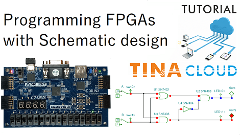
Creating Macros from Verilog using TINACloud (updated tutorial video)

Creating Macros from Verilog using TINACloud (updated tutorial video)

In this tutorial video we will show you how you can create a macro from a Verilog (.v) code and use in TINACloud.

You can create macros from VHDL, Verilog-A and Verilog-AMS files in a similar way.

The essential Verilog code of the half adder is 2 lines long only. The Verilog code is much simpler than the equivalent VHDL code. This is one of the great advantages of Verilog.

Similarly to our previous video “Creating Macros from VHDL” we will represent how you can turn the uploaded Verilog file into a Verilog macro. and we demonstrate how to Edit the Macro Input and Output pin names.

If you wish you can move the pin names to the top or to the bottom fields of the editor you can create pins at the top or at the bottom of the macro box.

Of course you can also change the names, for example A to Inp A, B to Inp B and so on.

Finally we will test our newly created macro in TINACloud’s Digital interactive mode along with the previously created VHDL macro and compare the results with the Truth Table of the Half Adder.

Watch our tutorial video to learn more.

You can learn more about TINA here: www.tina.com

You can learn more about TINACloud here: www.tinacloud.com

Creating Macros from VHDL using TINACloud (updated tutorial video)

Creating Macros from VHDL using TINACloud (updated tutorial video)

Hardware Description Languages are powerful tools to describe and simulate complex electronic devices.

In this tutorial video we will show you how you can create a macro from a VHDL (.vhd) code and use in TINACloud.

First we will select a file which we will turn into a VHDL macro from the original folder of the off-line TINA, but you can select a VHDL file anywhere on your computer.

By default, the input ports of the interface will appear on the left side of the generated macro shape and the output ports of the interface will appear on the right side. However by editing the generated macro you can change this arrangement. We will demonstrate how you can edit the Macro Input and Output pin names using the “Edit Macro Pins” display window of TINACloud.

Next, we will test our macro in TINACloud’s Digital interactive mode and compare the results with the Truth Table of the Half Adder. To do this we will place two High-Low Digital Switches from the Switches Toolbar, one for each of the A, B inputs and two Logic Indicators.

Watch our updated tutorial video to learn more!

You can learn more about TINA here: www.tina.com

You can learn more about TINACloud here: www.tinacloud.com

Adding SPICE models to TINA and TINACloud

Adding SPICE models to TINA and TINACloud

We are often asked about adding Spice models to TINA. Here are some tutorial videos about this topic:

Creating Subcircuits from Spice Models in TINA: .MODEL format

Creating Subcircuits from Spice Models in TINACloud: .MODEL format

Creating Subcircuits from Spice Models in TINA MODEL format

Click the picture to start video tutorial.


Click the picture to start video tutorial.

In these videos  we will present how to create your own component with TINA and TINACloud
therefore we will use the Spice model of  the BC846 NPN Bipolar transistor given in .Model format.

Creating Subcircuits from Spice Netlists in TINA, part 1: Simple 5-terminal Operational Amplifiers

Creating Subcircuits from Spice Netlists in TINA, part 2: Complex multi-terminal Op Amps

Creating Subcircuits from Spice Netlists in TINA, part 1 Simple 5-terminal Operational Amplifiers-Blog

Click the picture to start video tutorial.

In this tutorial video we will create an UA741 Operational Amplifier model using a  Spice Subcircuit in TINA.

Creating Subcircuits from Spice Netlists in TINA, part 2 Complex multi-terminal Op Amps-blog

Click the picture to start video tutorial.

In this tutorial you can learn how to create a  TINA macro component using a THS4121 Spice Subcircuit (downloaded previously from the net).

Creating Subcircuits from Spice Netlists with TINACloud


Click the picture to start video tutorial.

Watch this tutorial and learn how to create a TINA macro component using a THS4121 Spice Subcircuit with TINACloud.

You can learn more about TINA here: www.tina.com

You can learn more about TINACloud here: www.tinacloud.com

RLC rezgőkör létrehozása és szimulációja a TINA programban (Creating and simulating an RLC resonator circuit using TINA)

RLC rezgőkör létrehozása és szimulációja a TINA programban (Creating and simulating an RLC resonator circuit using TINA)
The rest of this blog is in Hungarian language.
You can find the English version here:

Creating and simulating an RLC resonator circuit using TINA

Ebben az oktatóvideóban egy RLC rezgőkör létrehozását és szimulációját mutatjuk be a TINA program segítségével.

Az TINACloud  oktatóvideóhoz hasonlóan itt is először létrehozzuk az RLC áramkört, ezt követően beállítjuk a szükséges alkatrész paramétereket, majd teszteljük az áramkört.

Az Ellenállás (R1) értékét 200 Ω-ra  állítjuk be, a Kondenzátort (C1) 1nF-ra.

A továbbiakban többféle módon is teszteljük az RLC áramkört, melyek a következők:
  1. Tranziens analízis
  2. Szimbolikus analízis
  3. AC analízis

A TINA programban a szimulációs eredmények (diagramok) beilleszthetőek a szerkesztési felületre, így az áramköri rajz és az áramkör analízis eredményei együtt tárolhatók.

Az oktatóvideóban többek között azt is bemutatjuk, hogy hogyan lehet a diagramokat, képleteket hozzáadni a kapcsolási rajzhoz.

Szó lesz arról is, hogy hogyan lehet a TINA programban a szimbolikus analízis során generált képleteket testreszabni, illetve címet is adunk az áramköri file-nak.

Videónk a következő linkre kattintva érhető el: RLC rezgőkör.

Az alábbi weboldalakon érhet el minket:

www.tina.com

www.tinacloud.com

Youtube elérhetőségünk: https://www.youtube.com/user/TinaDesignSuite

Félösszeadó áramkör szimulációja a TINA programban (Simulation of a Half Adder using TINA)

Félösszeadó áramkör szimulációja a TINA programban (Simulation of a Half Adder using TINA)
The rest of this blog is in Hungarian language. You can find the English version here
1. Félösszeadó kapcsolási rajzának létrehozása

Az alábbiakban egy félösszeadó áramkör létrehozását és szimulációját mutatjuk be a TINA program segítségével.

Ez az oktatóvideó mind az Európában használatos IEC mind pedig az amerikai ANSI szimbólumokkal is elkészült, melyek az alábbi linkekre kattintva érhetők el:

Oktatóvideó: IEC

Oktatóvideó: ANSI

Megjegyezzük hogy logikai komponensekre az amerikai ANSI szimbólumokat Európában és Magyarországon is sokan kedvelik.

Természetesen a TINA és TINACloud programokban bármikor átválthatunk a két szimbólumkészlet bármelyikére.

Először létrehozzuk a félösszeadó kapcsolási rajzát. A Sum (összeg) előállításához KIZÁRÓ-VAGY kaput, míg az Carry (átvitel) előállításához ÉS kaput használunk. Bemeneteket High-Low alternatív kapcsolók segítségével állítjuk elő.

2. Félösszeadó áramkör tesztelése DIG Interaktív gomb segítségével

Miután létrehozzuk a Félösszeadó kapcsolási rajzát, teszteljük áramkörünket a DIG Interaktív Digitális gomb megnyomásával.

Abban az esetben, ha a programban más interaktív mód lenne beállítva, akkor kattintsunk az Interaktív menüpontra, és a legördülő listából válasszuk ki a Digitális opciót.

Az interaktív módot úgy is kiválaszthatjuk, ha a  DIG interaktív ikon mellett található kis nyílra kattintunk, majd a  legördülő listából választjuk ki a Digitális opciót.

3. Alternatív kapcsolók helyettesítése egy-egy digitális jelgenerátorral

Ezt követően töröljük mindkét alternatív kapcsolót, és egy-egy digitális jelgenerátorral helyettesítjük azokat.

Az összes jelkombináció generálásához 1s időtartamon beállítjuk először a PS1 Digitális Jelgenerátor értékét magas (H) logikai szintre 0.2s és 0.6s között, majd a PS2 Digitális Jelgenerátor értékét 0.4s és 0.8s közötti magas logikai szintre.

Ezek után hozzáadunk még az áramkörünk Bemenetéhez két Kimenetet, hogy a szimulációs eredményeket bemutató diagramunkon a bemeneti jelek is láthatóvá váljanak.

4. Újonnan hozzáadott Kimenetek átnevezése, és sorrendiség meghatározása a diagramban

Átnevezzük az újonnan hozzáadott kimeneteket A-ra és B-re. Még
mielőtt lefuttatnánk a diagramot, meghatározzuk a sorrendiséget.

Ehhez A-t átnevezzük. A:1-re, a B kimenetet B:2-re és a Sum-ot Sum:3-ra.

Ezekkel a beállításokkal tehát meghatározhatjuk a jelek sorrendjét a diagramon A lesz legfelül, ezt követi B, Sum és Carry.

5. Az áramkör tesztelése Digitális Analízis segítségével

Oktatóvideónk végén teszteljük áramkörünket Digitális Analízis segítségével.

A kapott diagramban minden jel külön és a megadott sorrenben szerepel.

Nézze meg videóinkat, melyek az alábbi linkekre kattintva érhetők el.
IEC
ANSI 

A következő weboldalakon érhet el minket:

www.tina.com

www.tinacloud.com

Youtube elérhetőségünk: https://www.youtube.com/user/TinaDesignSuite