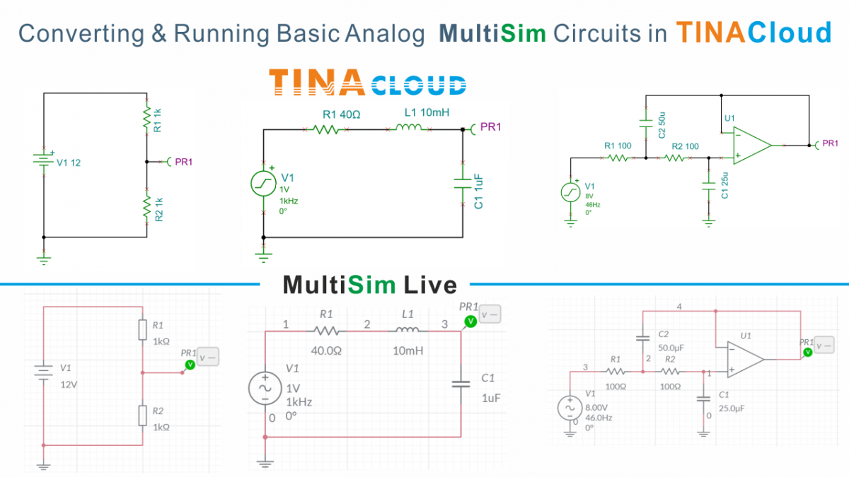
With the announcement that the Multisim Live simulator will be shut down on September 15, 2026, many engineers, educators, and students are looking for a reliable online alternative to continue their work.
TINACloud offers a seamless transition path, allowing you to import, run, and analyze circuits created in Multisim v14.2 and Multisim Live. In this guide, we will walk through the process of converting analog circuits and exploring the advanced analysis features—like symbolic analysis—that TINACloud brings to your projects.
Click here or on the image above to watch this blog presented as a video tutorial.
1. Exporting Your Design from Multisim Live
Before moving to TINACloud, you need to retrieve your files from the Multisim Live environment.
- Open your desired circuit (e.g., a “Voltage Divider”) in Multisim Live.
- Verify the design by clicking the Run button.
- Once verified, stop the simulation and navigate to the Menu.
- Select Download to save the circuit file to your computer.
2. Importing to TINACloud
TINACloud is designed to be compatible with various Multisim formats, including .ms14, .ms13, and the Multisim Live format, .msjs.
- Step 1: Log into TINACloud and select Upload from the menu.
- Step 2: Locate your downloaded
.msjsfile and select it. - Step 3: The circuit will appear in the TINACloud workspace, maintaining the original layout and parameters.
Voltage divider Circuit Analysis in TINACloud
Along with numerical analysis, TINA and TINACloud feature advanced capabilities such as symbolic analysis – a particularly powerful aid in teaching, as it brings to light the theoretical relationships that give meaning to the numerical values.
To see this in action, go to the Analysis menu, select Symbolic Analysis, and choose Symbolic DC Result. TINACloud will return the mathematical formula for the output voltage, providing clarity that a simple numerical value cannot.
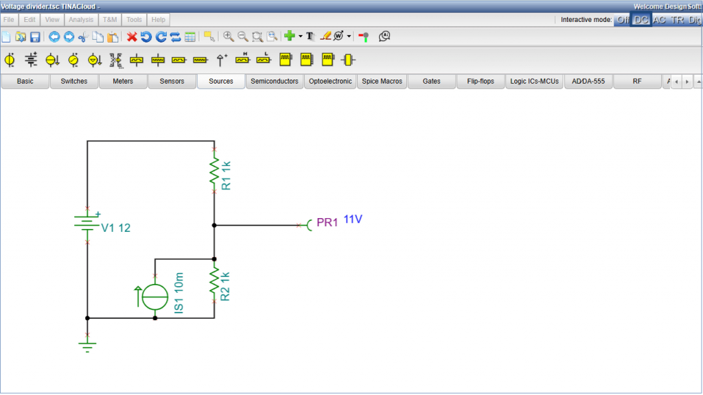
Analyzing a more complex circuit
Of course, Symbolic Analysis is not limited to simple circuits – it handles more complex ones just as well.
To see this, select Current Source from the Sources component toolbar, rotate it by 180 degrees, add it to the circuit, and connect it in parallel with R2. Then perform a numerical analysis first and repeat the calculation using Symbolic Analysis.
To obtain the numerical result, press the DC button.
Analyzing a more complex circuit
To obtain the symbolic result, follow the same menu path as before: Analysis > Symbolic Analysis > Symbolic DC Result.
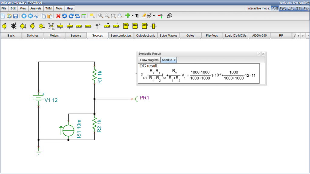
The program returns the analytical formula, which produces the same result as the numerical calculation. The formula clearly demonstrates the application of the superposition theorem, expressing the total response as the sum of the partial responses due to the current source and the voltage source acting independently. This is what makes symbolic analysis such a valuable teaching tool: it exposes the inner structure of the calculation, which is otherwise lost in a purely numerical answer.
Series RLC Circuit Analysis in TINACloud
We have already opened the circuit in Multisim Live and downloaded the file to our computer.
After launching TINACloud, let’s upload the file using the standard upload procedure. The schematic will appear, maintaining the same layout and parameters as seen in Multisim Live.
Numerical Analysis: Transient Analysis, AC Analysis
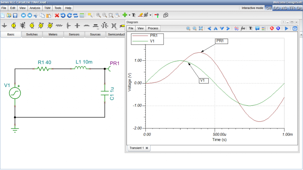
Transient Analysis
Numerical analysis allows us to observe the circuit’s behavior over time and frequency through data-driven simulations.
Let’s first run a Transient Analysis. To generate curves, run transient analysis via the Analysis menu\Transient…
The curves will appear in a single, shared diagram. The coordinate system magnifies the view between the minimum and maximum values.
Round the axis scales for better readability: Click an axis to open the scale settings. Select the Round axis scale checkbox, then click OK.
To view multiple curves simultaneously, go to the View menu and select “Collect curves“.
Enhance your results by adding a legend or individual labels to identify each curve.
AC Analysis
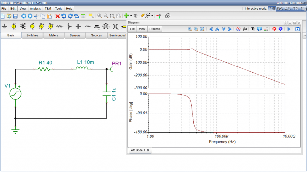
Now, let’s run AC Analysis. Navigate to the Analysis menu, select AC Analysis, then click AC Transfer Characteristic...
You can select several diagrams from the list. Select the Amplitude and Phase (Bode)diagrams. A two-panel Bode diagram will appear. As with the transient analysis, you can round the axis scales for clarity.
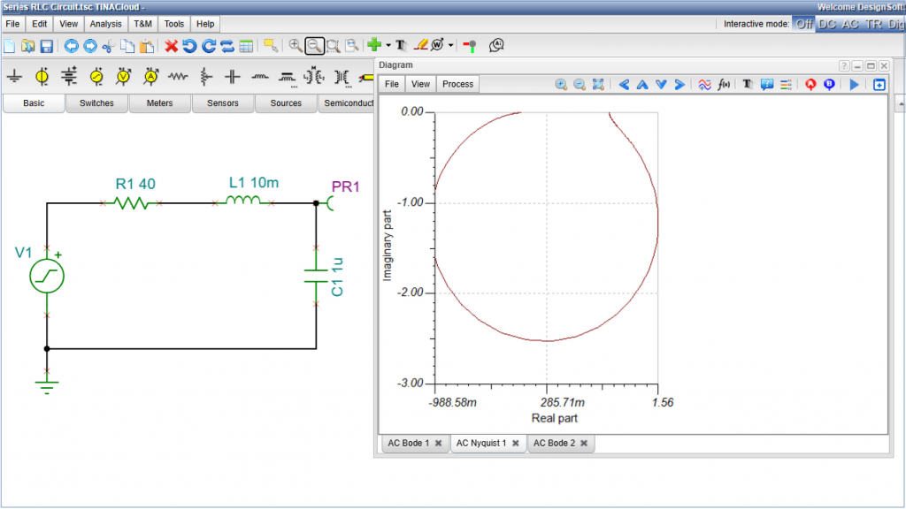
To perform other types of analysis, return to the Analysis menu and select AC Analysis > AC Transfer Characteristic… From there, you can choose Nyquist in the Analysis window to generate the diagram. To improve the resolution of the plot, increase the number of points (e.g., from 100 to 1000) and click Run. The Nyquist diagram appears. Adjust the axis scales as needed.
Symbolic Analysis
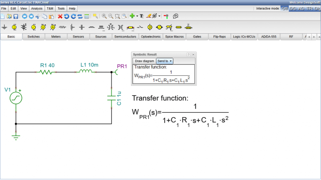
Beyond numerical data, TINACloud can perform symbolic analysis to generate mathematical formulas that describe your circuit’s behavior. Go to the Analysis menu, select Symbolic Analysis, then choose Symbolic AC Transfer. The transfer function will be displayed in its symbolic form, providing a direct analytical representation of the circuit’s performance.
The Text Editor allows you to embed the symbolic formula within the circuit design.
2nd Order Low Pass Filter Analysis
in TINACloud
For our third example, we will analyze a 2nd Order Low Pass Filter. Follow the standard procedure to download the circuit file from Multisim Live and upload it to TINACloud.
Transient Analysis
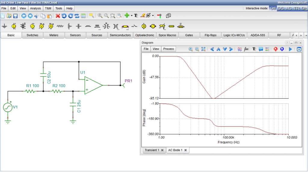
First, let’s perform a Transient Analysis. Navigate to the Analysis menu and select Transient. In the settings window, set the End Display time to 100m and press Run. The results will display the output (PR1) alongside the excitation signal (V1).
To view both signals in a single plot, go to View > Collect Curves.
Using the Virtual Oscilloscope
To observe the signals in real-time, we can use the built-in Oscilloscope.
Close the current diagram.
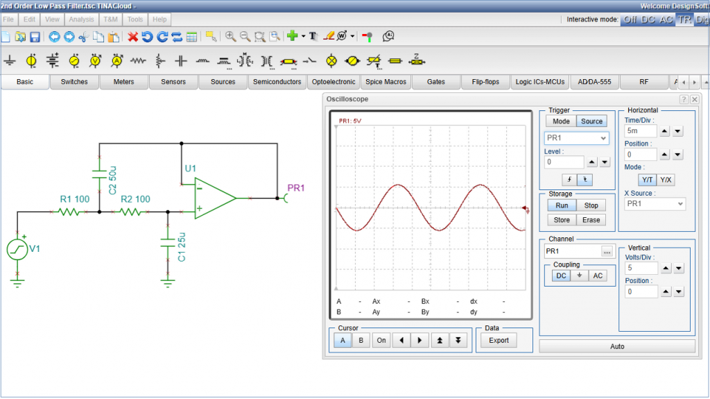
Go to the T&M (Test and Measurement) menu and select Oscilloscope.
Click Run and apply the following settings to clarify the signal: Set the Time/Div to 20ms and the Volts/Div to 5V. Adjust the Time/Div to 5ms for a more detailed view. To stabilize the waveform, change the mode from Auto to Normal. Under the Source tab, select PR1 as the trigger signal. You can now synchronize using either the positive or negative slope. Once finished, stop the simulation and close the Oscilloscope window.
AC and Symbolic Analysis
AC Analysis
Now, let’s examine the frequency response. Go to Analysis > AC Analysis > AC Transfer Characteristic… Go to Analysis > AC Analysis > AC Transfer Characteristic… Both the Amplitude and Phase curves will appear.
Transitioning to Symbolic Analysis
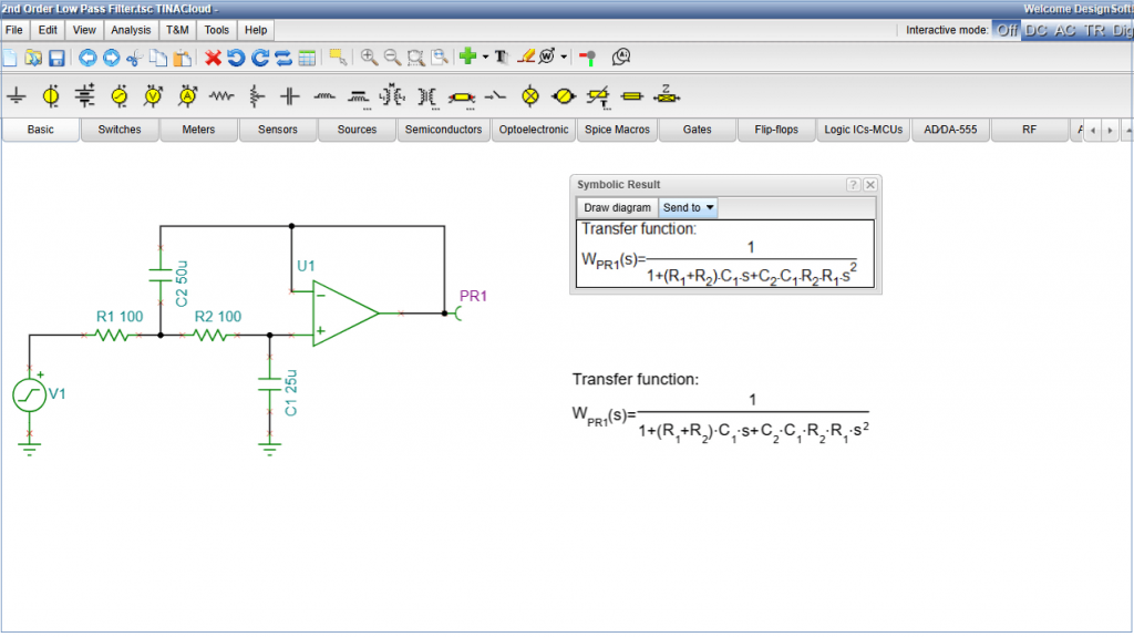
Because a standard Op-Amp is a non-linear component, TINACloud must treat it as an Ideal Operational Amplifier to generate a mathematical formula.
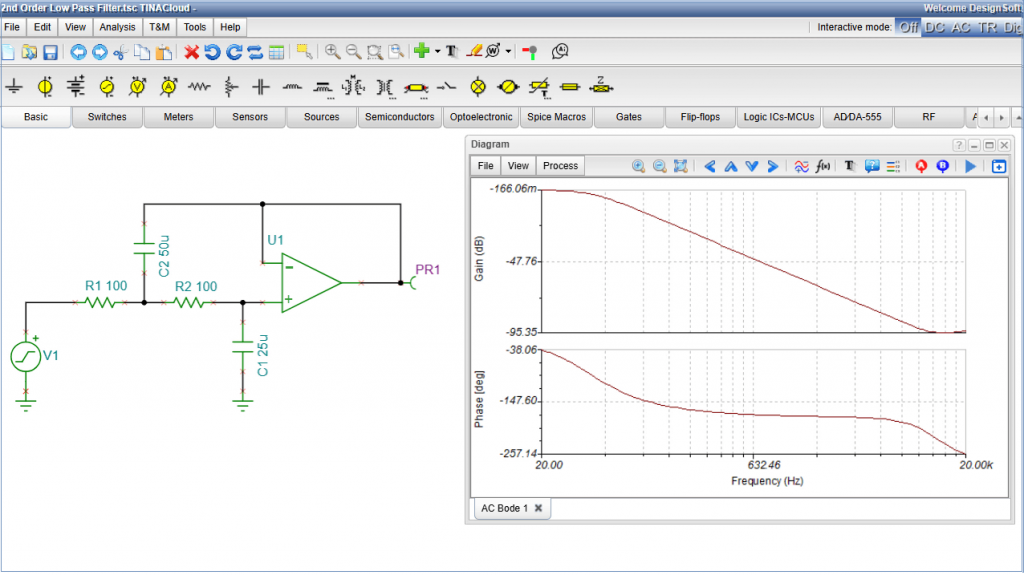
Let’s first recalculate the transfer characteristics numerically in a relevant voice frequency range.
Run AC Transfer Characteristic again specifically for the voice frequency range (20Hz to 20kHz) with 100 points.
The Bode plots (Amplitude and Phase) are displayed.
Now close the diagram and generate the formula. Go to Analysis > Symbolic Analysis > Symbolic AC Transfer. The Symbolic Transfer Function appears.
To add the resulting formula to your design, select the “Send to” tab and click “Text Editor” in the results window.
Check the text size, then click OK. The symbolic transfer function is now embedded in your schematic.
Comparing Ideal vs. Non-Linear Models
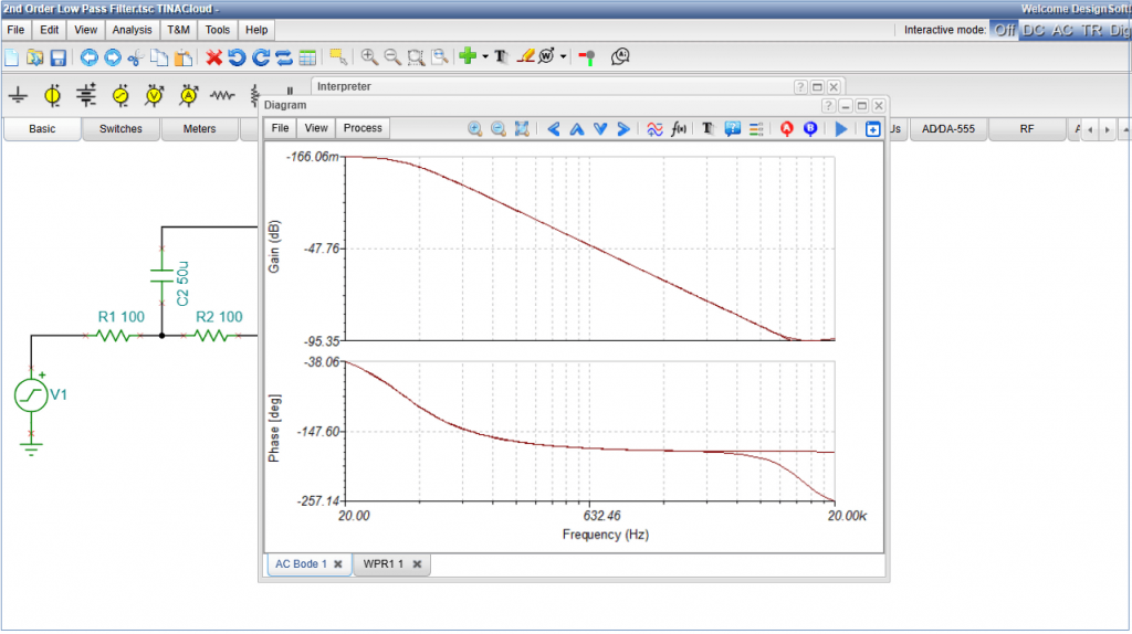
Finally, we can verify the accuracy of the ideal model by comparing it to the non-linear version. Open the Interpreter and press Run. This draws the transfer function based on the ideal model. Overlay this plot onto the existing Bode diagram to compare it with the non-linear model.
Click the curve and select the “Copy Curve“icon to copy it to the clipboard. Next, switch to the AC Bode Diagram tab, click on the plot area, and select the “Paste curve” icon. As you can see, the two curves match almost perfectly. The same is true for the phase characteristics, so let’s perform that comparison as well. Again, the agreement between the results is good; however, at higher frequencies the ideal op-amp shows deviations from the phase response of the more accurate nonlinear model.
That brings us to the end of this tutorial on converting basic Multisim Live circuits and running them in TINACloud.
Be sure to check out our other videos on logic circuits and more advanced topics.
Conclusion
Transitioning from Multisim Live doesn’t have to mean starting from scratch. TINACloud provides the tools to not only replicate your current work but to enhance it with symbolic formulas and integrated test equipment.
As the 2026 deadline approaches, we encourage you to begin migrating your libraries to ensure your projects remain accessible and functional in a cloud-based environment.
You can learn more about TINACloud here: www.tinacloud.com
Explore more content from our channel: https://www.youtube.com/@TinaDesignSuite