We are delighted to roll out a dedicated Chinese-narrated version of our core overview video, “What is TINA and TINACloud.” Serving a community of over 100,000 engineers, educators, and students across 200 countries, TINA and TINACloud deliver a powerful, cost-effective platform for advanced electronic circuit simulation and PCB design.
我们很高兴推出核心概览视频《What is TINA and TINACloud》的专属中文配音版本。TINA和TINACloud服务于全球200个国家、超过10万名工程师、教育工作者和学生,为高级电子电路仿真和PCB设计提供了一个功能强大且极具性价比的平台。
To ensure seamless access for all our users, this video is available on both platforms:
Flexible Deployment Options: Discover traditional offline desktop installations for Windows, macOS, major Linux distributions, and Raspberry Pi OS, alongside the browser-accessible, zero-installation TINACloud.
Integrated AI Support: Learn how native AI tools streamline engineering tasks, circuit design, and automation. The desktop version offers hardware acceleration—supporting NVIDIA, AMD, and Intel Arc GPUs—for secure, local model execution.
Comprehensive Circuit Analysis: Review capabilities covering analog, digital, mixed-signal, RF, microwave, and switched-mode power supply circuits, backed by support for over 1,400 microcontrollers (including the ESP32 family) and major Hardware Description Languages (such as VHDL, Verilog, and SystemVerilog).
Integrated PCB Design & 3D Visualization: Watch a concise demonstration of seamless schematic capture, layout creation, and realistic 3D rendering, including support for flex PCBs.
Whether you are an experienced circuit designer, an educator, or a student, this video outlines how TINA and TINACloud can streamline your design workflow and complex circuit analysis.
Explore More Tutorials and Videos
If you are interested in learning more about specific features of TINA and TINACloud, check out our additional resources:
We are pleased to announce the release of our comprehensive technical overview video, “What is TINA and TINACloud,” now live on YouTube with complete Vietnamese narration.
Trusted by over 100,000 engineers, educators, and students across 200 countries, TINA and TINACloud provide a robust, cost-effective ecosystem for advanced electronic circuit simulation and PCB design.
Chúng tôi rất vui mừng thông báo việc phát hành video tổng quan kỹ thuật toàn diện có tựa đề “TINA và TINACloud là gì” (“What is TINA and TINACloud”), hiện đã chính thức có mặt trên YouTube với phần thuyết minh hoàn toàn bằng tiếng Việt.
Được tin dùng bởi hơn 100.000 kỹ sư, giảng viên và sinh viên tại hơn 200 quốc gia, TINA và TINACloud mang đến một hệ sinh thái mạnh mẽ, tối ưu chi phí dành cho việc mô phỏng mạch điện tử tiên tiến và thiết kế PCB.
Key Highlights Covered in the Video:
Flexible Deployment Options: Explore offline desktop installations—supporting Windows, macOS, major Linux distributions, and Raspberry Pi OS—alongside the browser-based, zero-installation TINACloud.
Integrated AI Support: Discover how built-in AI tools assist with engineering tasks, circuit design, and automation. The offline version features hardware acceleration (supporting NVIDIA, AMD, and Intel Arc GPUs) for local, privacy-focused model execution.
Comprehensive Circuit Analysis: Learn about capabilities spanning analog, digital, mixed-signal, RF, microwave circuits, and switched-mode power supplies, alongside support for over 1,400 microcontrollers (including the ESP32 series) and major Hardware Description Languages (VHDL, VHDL-AMS, Verilog, Verilog A&AMS, SystemVerilog, SystemC).
Integrated PCB Design & 3D Visualization: A brief demonstration of seamless schematic capture, layout design, and 3D rendering (including flex PCBs).
Whether you are an experienced circuit designer, an educator, or a student, this video outlines how TINA and TINACloud can streamline your design workflow and complex circuit analysis.
International Exhibition & Conference for Educational Resources, Technology, and Skills Development
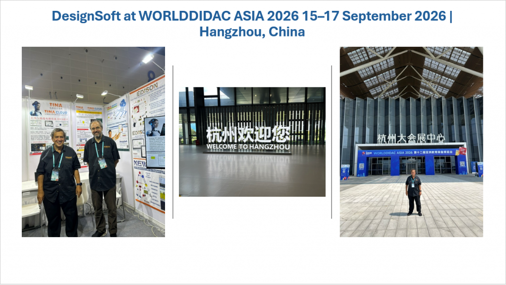
We are exhibiting at Worlddidac Asia 2026, an international exhibition and conference for educational technology, teaching resources, and skills development, taking place in Hangzhou, China, from 15–17 September. The event brings together education authorities, universities, schools, distributors, and technology providers from across Asia and beyond. It features innovative solutions for K–12, vocational training, and higher education, with a strong focus on AI, STEM, digital transformation, laboratory technology, and practical skills development.
DesignSoft at WorldDidac Asia 2026
DesignSoft at WorldDidac Asia 2026-First day /Hall 8, booth C13 /
Visit us in Hall 8, booth C13!
We are showcasing the latest versions of TINA and TINACloud, along with our newest innovations, including:
Enhanced cross-platform support: now available for Windows, Apple OS, and major Linux distributions (Ubuntu, Mint, SUSE, Raspberry Pi, and more).
Dark mode support: optional black background for schematics and simulation results
Support for Foldable Phones
TINACloud runs smoothly on the Samsung Galaxy Z Fold 8 and Z Fold 8 Ultra.
Support for additional foldable phones is currently being tested.
Powerful Import and Conversion Tools:
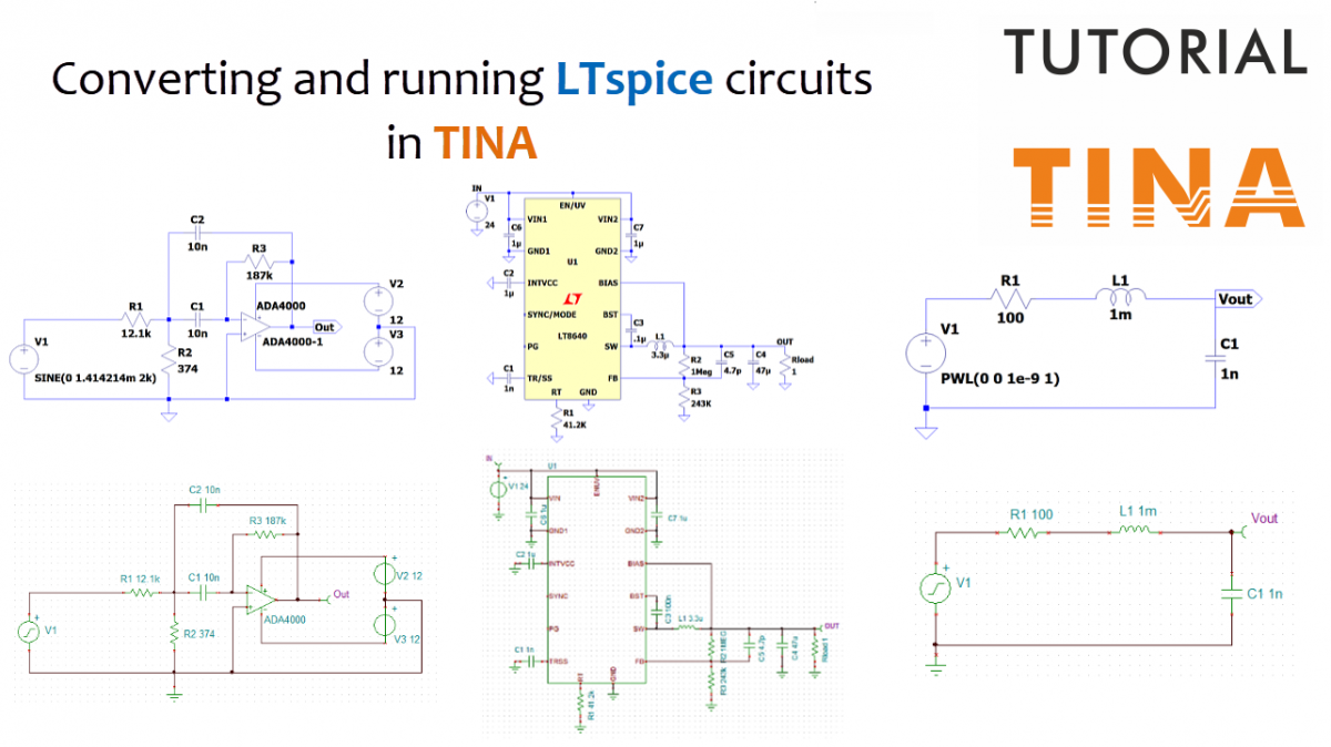
Converting LTspice, Multisim, Multisim Live, and Proteus projects to TINA and TINACloud.
Harmonic Balance: New analysis method for RF and Microwave circuits
Harmonic Balance Analysis of: MW mixers, modulators, demodulators, and more…
New Microcontroller models
ESP32C3, ESP32S3
AI improvements:
Fast offline LLM models
Support for LM Studio
Speech support
Support for AMD GPUs, Intel Arc GPUs
Improvements in the AI AC/DC solver
Improved AI Supported Filter Design
More AI supported Oscillator Circuits
Python code generation using multiple LLMs (ChatGPT, Copilot, Claude, DeepSeek, and more)
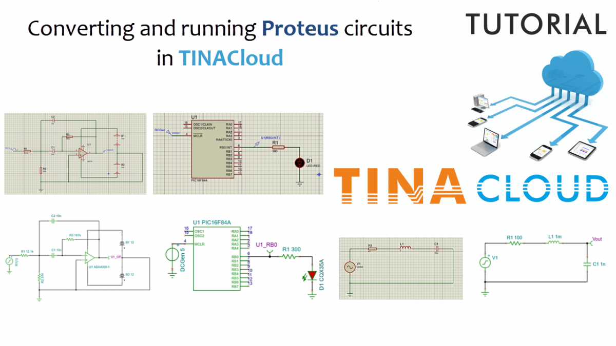
In this post, we will show you how to seamlessly convert Proteus circuits into TINACloud.
By converting these circuits into TINACloud, you can instantly run and analyze them anywhere-without any installation-on virtually any device, including PCs, laptops, tablets, and smartphones, regardless of the operating system, whether it’s Windows, macOS, iOS, Android, or more. All you need is a modern web browser.
It is important to note that this conversion process is also available in the offline version of TINA, allowing you to perform the transition locally.
The resulting .TSC files are fully cross-compatible, providing a seamless workflow between the offline desktop software and the online TINACloud environment.
Click hereor on the image above to watch this blog presented as a video tutorial.
Example 1: Educational RLC Circuit
TINACloud includes several ready-to-use sample circuits, which you can find under the Examples/3rd Party files/Proteus folder.
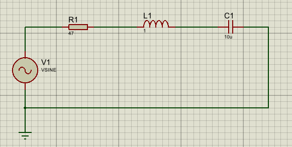
Let’s start with a simple educational RLC circuit. This is how the circuit looks in Proteus.
RLC circuit in Proteus
1. Importing the Circuit
Navigate to the Examples / 3rd Party files / Proteus folder.
Select the RLC circuit file (RLC.pdsprj) and click Open.
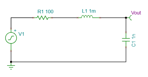
After conversion, the circuit is reproduced exactly in TINACloud, as shown here:
RLC circuit in TINACloud
2. Running a Transient Analysis
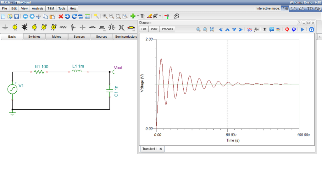
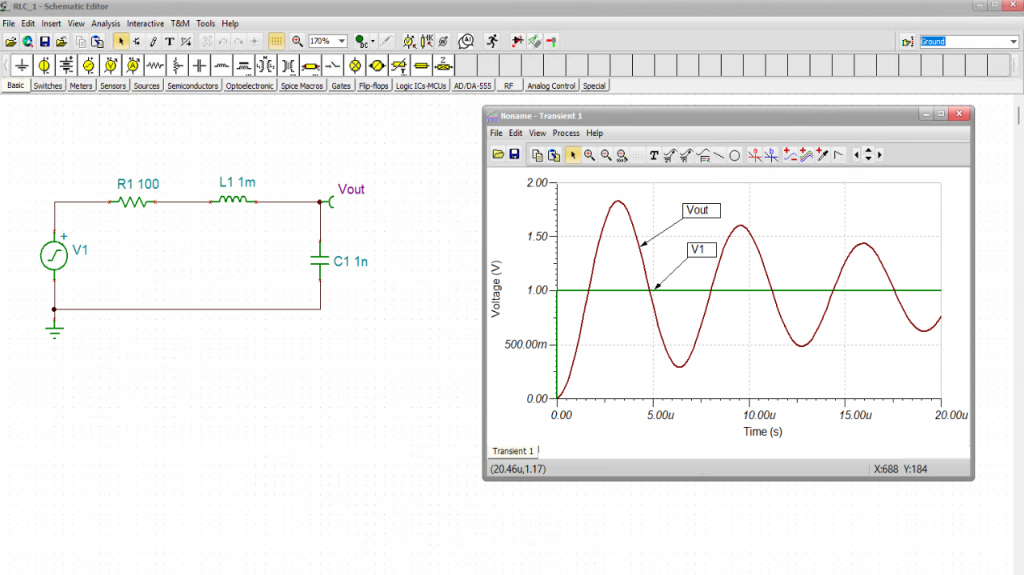
First, we will run a Transient Analysis. Go to the Analysis menu and select Transient… As soon as the simulation completes, the resulting time-domain waveforms are displayed cleanly on the screen.
Using the Collect Curves command from the View menu in the Diagram window, you can also plot the input and output waveforms on the same coordinate system.
You can also label the curves with their signal names using the Auto-Label Curves icon in the Diagram window.
RLC circuit in TINACloud: Transient analysis result
3. Configuring AC Analysis
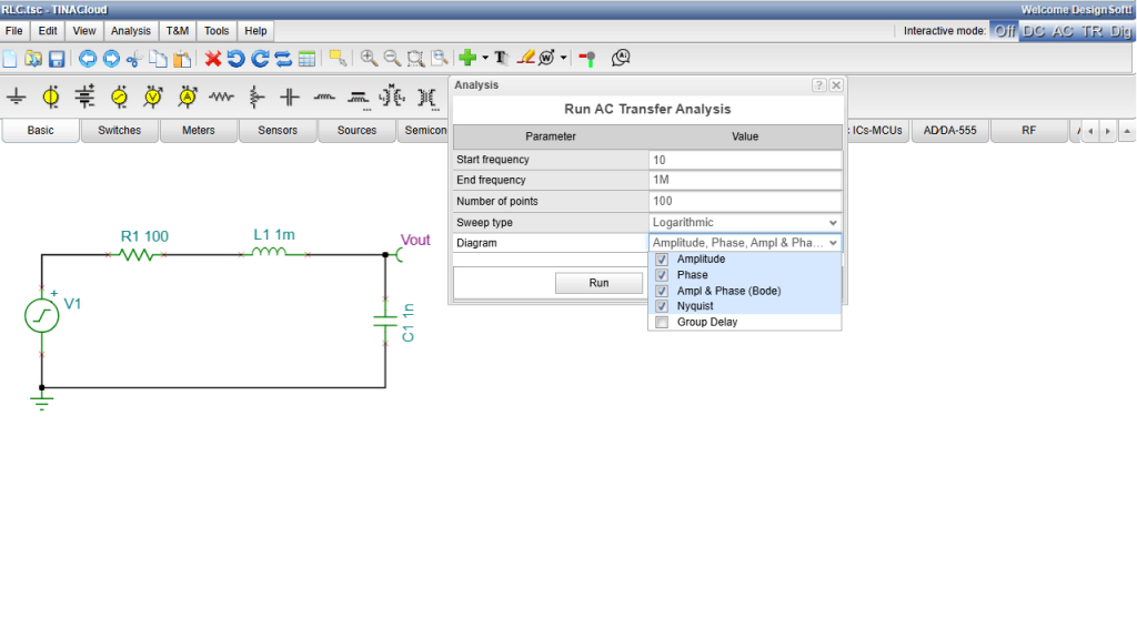
Next, let’s explore the frequency domain. Navigate to the Analysis menu and select AC Analysis >AC Transfer Characteristic…
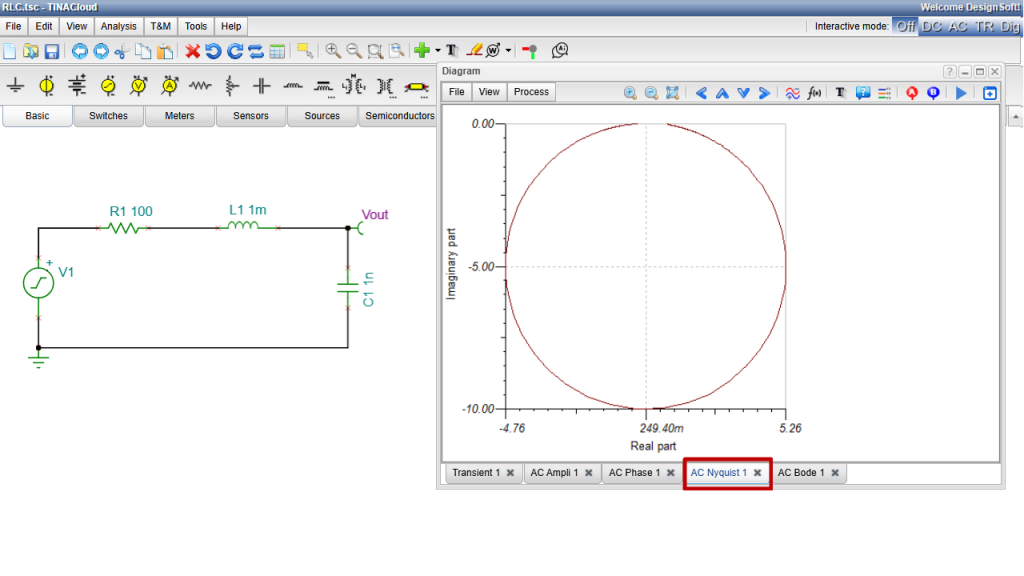
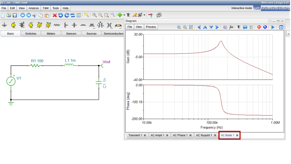
In addition to standard AC Bode plots, TINACloud features advanced calculation capabilities, allowing you to easily generate Amplitude, Phase, Nyquist, and Group Delay diagrams.
RLC circuit in TINACloud: Parameter settings before running AC Analysis
Select the AC Bode, Amplitude, Phase and Nyquist diagrams, and set the start frequency to 10 kHz and the number of points to 1,000 for a high-resolution output, then click Run to execute the analysis.
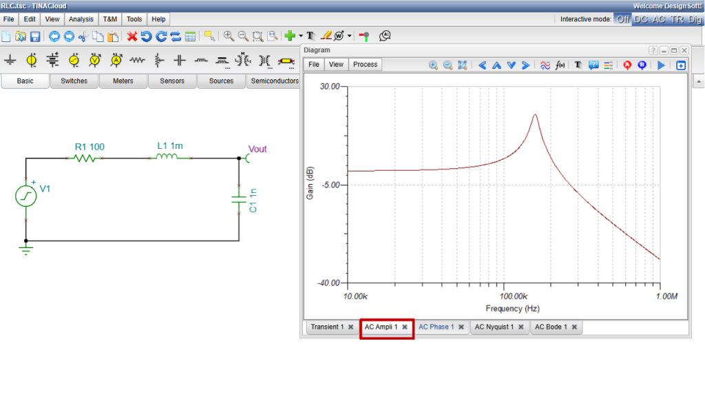
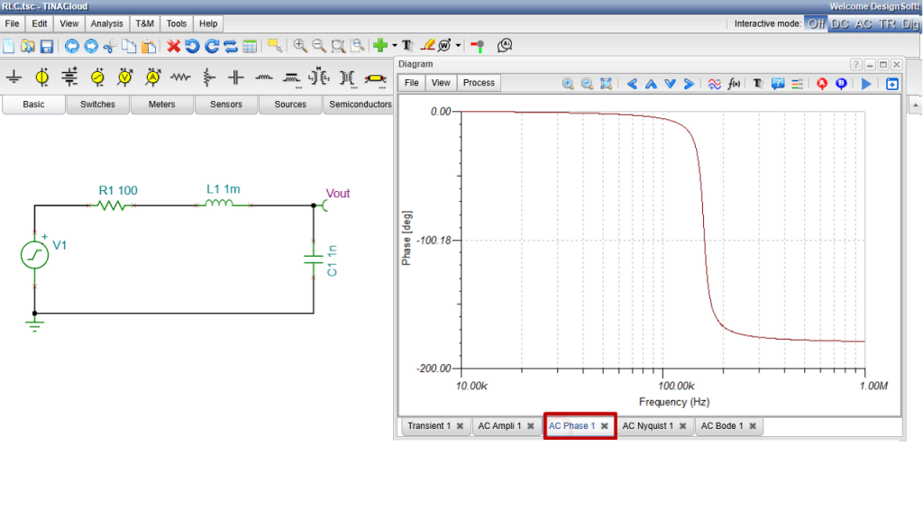
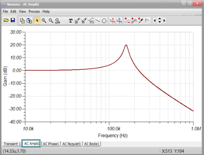
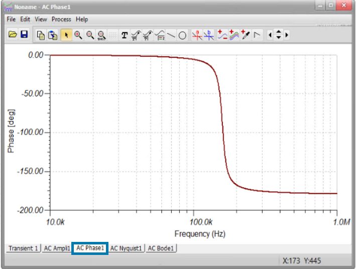
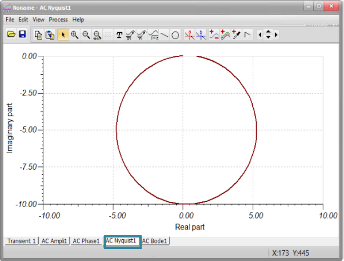
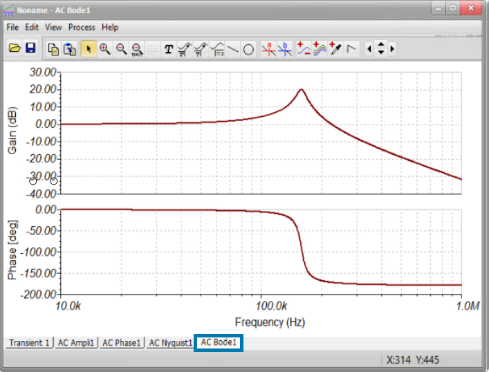
Four separate tabs will appear, displaying the Amplitude, Phase, Nyquist and Amplitude & Phase (Bode) diagrams.
RLC circuit in TINACloud: Amplitude diagram
RLC circuit in TINACloud: Phase diagram
RLC circuit in TINACloud: Nyquist diagram
RLC circuit in TINACloud: Bode diagram
4. Symbolic Analysis in TINA and TINACloud
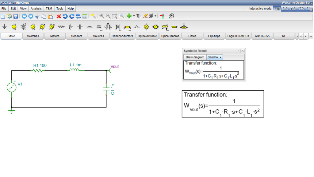
A unique feature of TINA and TINACloud is the ability to derive a circuit’s Transfer Function symbolically, presenting it as an exact mathematical formula. This allows engineers and students to gain deeper insights into circuit behavior-including poles, zeros, gain, and frequency response. This symbolic expression can also be used for analytical studies, documentation, optimization, and verification, moving beyond a sole reliance on numerical simulation results.
Note: While symbolic transfer function derivation is only possible for linear circuits, you can still analyze active filters implemented with op-amps. In TINA and TINACloud, nonlinear operational amplifier models are automatically replaced with ideal op-amp models during symbolic analysis. This provides highly accurate results, allowing the transfer function to be derived and analyzed symbolically.
Running Symbolic Analysis
To perform Symbolic Analysis, open the Analysis menu, select Symbolic Analysis, then Symbolic AC Transfer, and run the analysis.
The analytical form of the Transfer Function will immediately be displayed on your screen.
You can now insert the symbolic expression into the TINACloud Text Editor and place it directly onto the schematic, making the analytical results part of your circuit documentation. In the Symbolic Result window click on the “Send to” tab then select the “Text editor”.
Note that the formula can also be edited within the Text Editor, though we won’t cover those editing features in this tutorial.
Once the formula appears in the Text Editor, click OK. The formula is now attached to your cursor. Position it wherever you like on the schematic, and left-click to place it.
RLC circuit in TINACloud: Running Symbolic Analysis and adding the formula to the schematic
Plotting and Comparing Results
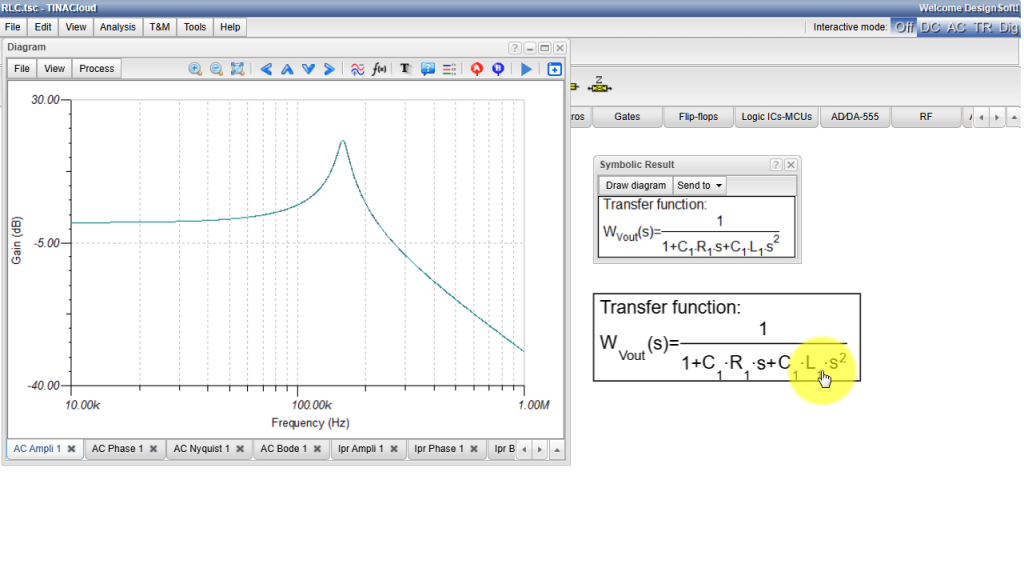
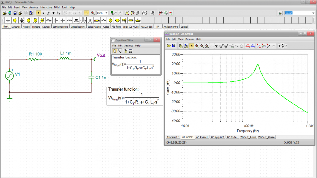
Beyond formulas, you can also plot the analytical transfer function to compare it directly with your numerical simulation results.
In the Symbolic Results window, simply click the Draw Diagram button. The plot of the Transfer Function will appear. To make comparing the analytical and numerical results easier, click on the curve and change its color to green. Next, click the curve again, then click the Copy curve icon to save it to your clipboard. Now, switch back to the previously calculated Ampl 1 tab, and use the Paste Curve icon to overlay the symbolic result directly onto the numerical curve.
As you can see, the two curves match perfectly within the line width.
RLC circuit in TINACloud: Comparing the analytical and numerical results
Example 2:Active Band-Pass Filter
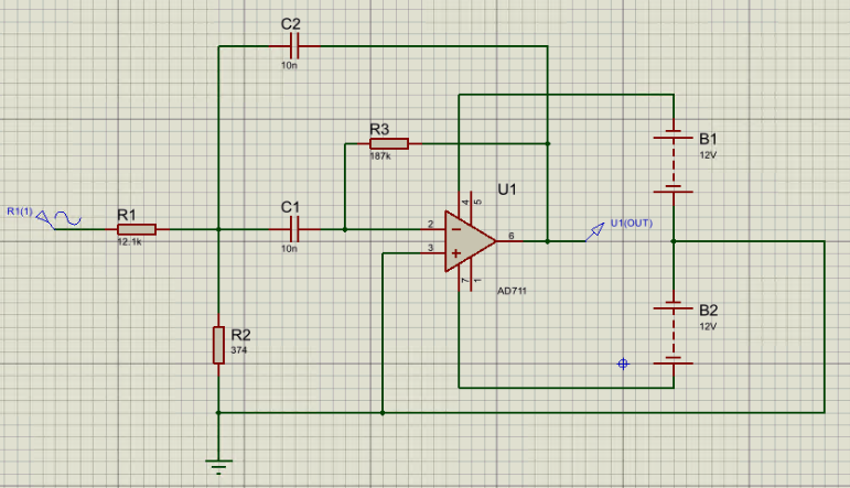
For our next example, we’ll look at a band-pass filter, built around the Analog Devices ADA4000-1 operational amplifier. This circuit is a standard building block for what we call active filters, and here is what it looks like in Proteus:
Active Band-pass filter circuit in Proteus
File Import and Conversion
To bring this into the TINACloud workspace, save the circuit to your local Downloads folder. Next, use the Upload command to convert the file.
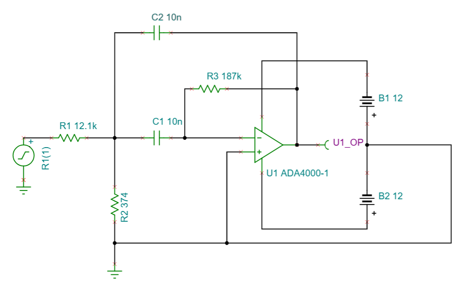
After conversion, the circuit is reproduced in TINACloud, as shown here.
Active Band-pass filter circuit in TINACloud
Next, save it as ‘Active Band-pass Filter.tsc’.
Running AC & Symbolic Analysis
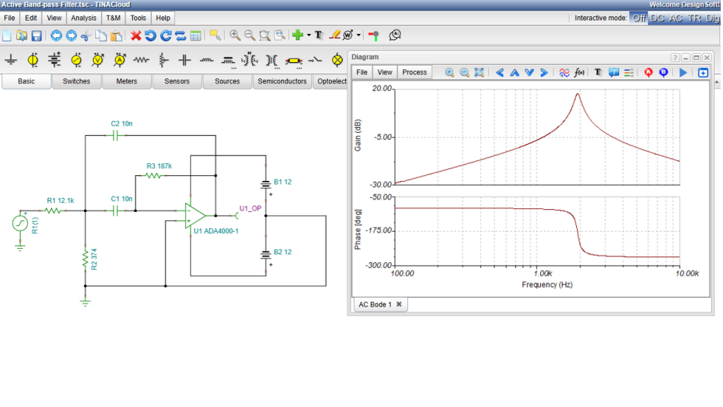
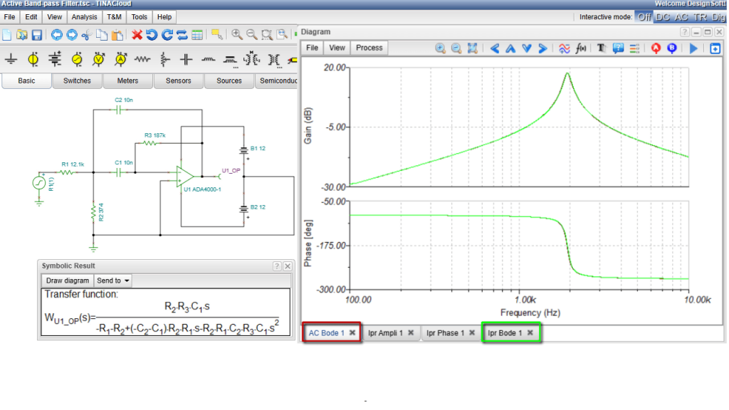
Since the setup is similar to our previous example, we’ll focus just on running the AC and Symbolic Analyses for this simulation. We’ll start with the AC Analysis, which generates our combined Amplitude and Phase Bode Plot.
Go to the Analysis menu, select AC Analysis, AC Transfer Characteristic. Click Run.
The combined Amplitude and Phase Bode Plot appears.
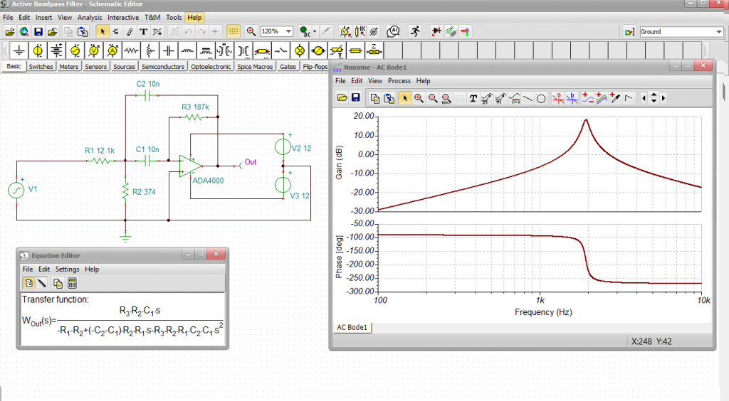
Active Band-Pass Filter circuit in TINACloud: AC Bode diagram
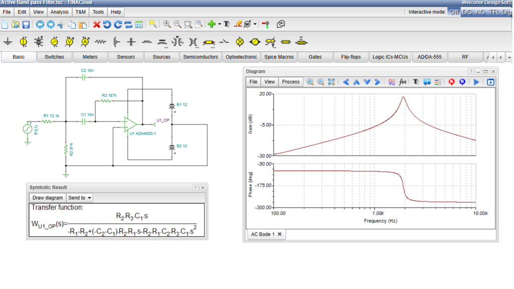
Next, run the Symbolic AC Transfer Analysis. Just as we explained in the last video, TINA and TINACloud automatically swap out the nonlinear ADA4000-1 for an ideal op-amp. This substitution makes symbolic analysis possible, allowing TINACloud to generate the analytical transfer characteristic.
Active Band-Pass Filter circuit in TINACloud: Symbolic analysis result
Plot Visualization
Now, let’s compare this analytical result with our numerically calculated Bode Plot. In the Symbolic Result window click the Draw Diagram tab. Three plots will appear: the Amplitude, the Phase and the combined Bode Plot.
Comparing and Overlaying the Curves
To easily compare the two methods, first change the color of the analytical Amplitude Plot to green, and copy the curve to your clipboard. Then, switch over to the numerically calculated Bode Plot tab, and paste the green curve directly into the Amplitude Plot.
Repeat this exact same procedure for the Phase Plot.
Final Analysis and Conclusion
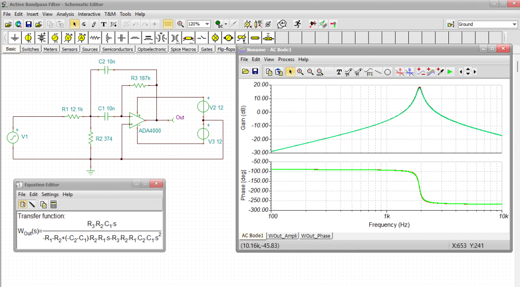
When you look at the results, you can see that the numerically calculated curves align perfectly with the analytical curves. As we’ve emphasized in previous videos, this excellent agreement demonstrates exactly why ideal operational amplifiers are so widely used in active filter synthesis.
Active Band-Pass Filter circuit in TINACloud: Comparing and Overlaying the Curves
Example 3: 8-bit PIC Microcontroller
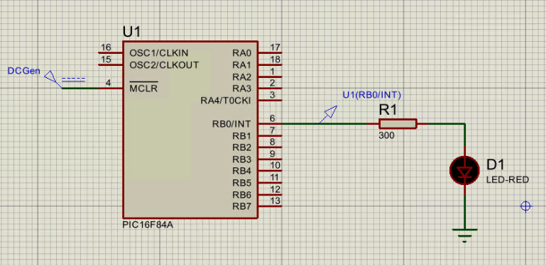
8-bit PIC Microcontroller in Proteus
Our final example features an 8-bit PIC Microcontroller (MCU). Here, we will demonstrate the conversion to TINACloud, but a very similar conversion process is also available in the offline version of TINA. The resulting .TSC files can be opened and run in both TINA and TINACloud.
The converted microcontrollers are fully operational in both the offline and cloud versions of TINA.
Now, open the PICLedBlink.pdsprj file from the TINA Examples\3rd Party files\Proteus folder.
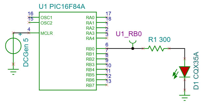
8-bit PIC Microcontroller in TINACloud
Once the conversion is complete, press the TR button, and you’ll see the LED begin to blink immediately. TINACloud also allows you to study the code execution using the built-in MCU Debugger:
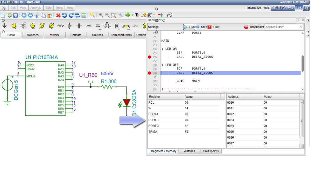
Enable MCU Code Debugger in the Analysis menu. Press the TR button again to launch the debugger window.
From here, you can use the Step button to execute code line-by-line while monitoring Registers and Memory.
You can also set Breakpoints by clicking on a line of code or using the Breakpoint button.
Press Run, and the program will halt at your designated points. Pay close attention to Port B, which directly controls the LED.
8-bit PIC Microcontroller in TINACloud-Using the Debugger
Programming MCUs in C
While Assembly is powerful, you can also program MCUs in TINACloud using C.
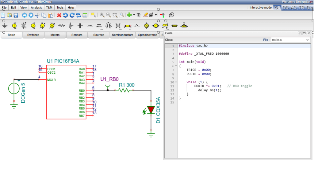
Let’s open the PICLedBlink_CCode.pdsprj file. This circuit looks identical to the previous one, but the PIC is running on C-code. Double-click the MCU, click the “…” at the end of the MCU-code line. Here you can upload your C code or preview existing code. For now, let’s preview the code that’s already been uploaded.
8-bit PIC Microcontroller in TINACloud-Preview of the C code
Note that in both TINA and TINACloud, C code can be debugged just like assembly code-either by executing it step by step or by using breakpoints.
In addition to PIC microcontrollers, TINA and TINACloud support more than 1,400 microcontrollers, including: AVR, 8051, HCS, ARM, Raspberry Pi, ESP32, ST, Arduino, XMC, and more.
Conclusion
This concludes our tutorial on converting Proteus circuits and running them in TINACloud. Please note that the same procedure also works in the offline version of TINA, and the resulting .tsc files are fully compatible with both TINA and TINACloud.
This post explores the workflow for migrating LTspice circuits (.asc files) into TINA, DesignSoft’s circuit simulator. We demonstrate how to import, execute, and evaluate these schematics locally on a computer. A key takeaway is the full cross-compatibility of the resulting .TSC files, which ensures a unified workflow between the TINA desktop application and the TINACloud platform.
Click here or on the image above to watch this blog presented as a video tutorial.
1. Importing and Basic Analysis (RLC Circuit Example)
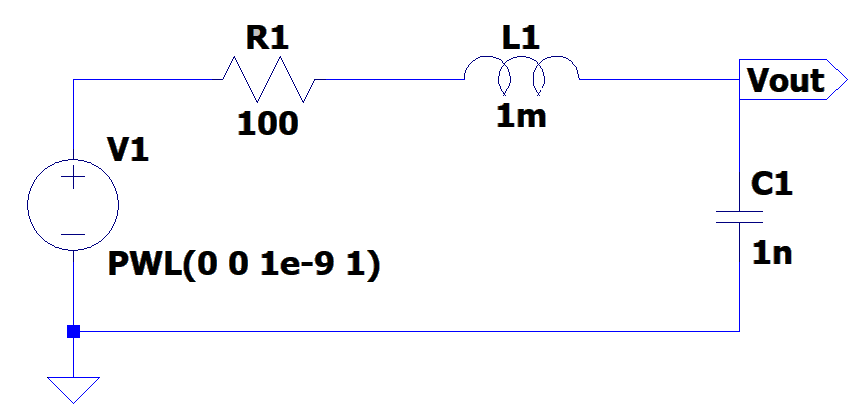
The conversion process is straightforward. By using the File > Import > LTspice command, users can bring LTspice designs into the TINA schematic editor. The tutorial demonstrates this using an educational RLC circuit.
RLC Circuit in LTspice
Transient Analysis
Once the schematic is imported, users can perform a Transient Analysis to examine the circuit in the time domain.
Visualization: Waveforms are displayed in a diagram window.
Customization: The “Collect Curves” function allows users to plot multiple signals (e.g., input and output) on the same coordinate system.
Identification: The “Auto-Label Curves” tool helps identify voltages and currents directly on the graph.
Displaying transient analysis waveforms in TINA, including overlaid input/output curves and custom signal labeling
AC Analysis
To explore frequency-domain behavior, the AC Transfer Characteristic is used. Beyond standard Bode plots, TINA provides:
Multi-Diagram Output: Users can generate Amplitude, Phase, Nyquist, and Group Delay diagrams simultaneously.
High-Resolution Results: By configuring start frequency and the number of plot points, users can generate detailed, high-resolution outputs across multiple tabs.
TINA AC analysis view: Amplitude diagram for the imported RLC circuit
TINA AC analysis view: Phase diagram for the imported RLC circuit
TINA AC analysis view: Nyquist diagram for the imported RLC circuitm
TINA AC analysis view: Bode diagram for the imported RLC circuit
2. Symbolic Analysis
Another highlight of the tutorial is the ability to derive a circuit’s Transfer Function symbolically as an exact mathematical formula. This provides insights beyond numerical simulation, assisting in documentation and verification
Analytical Verification: The tutorial demonstrates how to extract this formula via the Equation Editor and paste it directly onto the schematic.
Curve Comparison: Users can plot the symbolic transfer function and overlay it on numerical simulation curves. A perfect alignment between the two confirms the circuit’s behavior and the accuracy of the model.
Verifying AC analysis: overlaying numerical and symbolic amplitude plots for the RLC circuit
3. Active Filters and Operational Amplifiers
Using an active band-pass filter circuit based on the Analog Devices ADA4000-1 operational amplifier, the video shows how these analysis tools apply to standard building blocks.
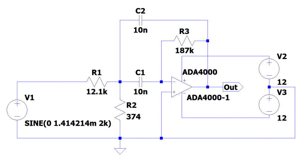
Active Band-pass filter (ADA4000-1) circuit in LTSpice
The workflow:
Import the circuit file.
Run AC Analysis to generate the combined Amplitude and Phase Bode Plot.
Run Symbolic Analysis to derive the analytical transfer function.
Overlay the analytical curves onto the numerical plots to verify that the results align.
Active band-pass filter analysis in TINA, displaying the combined AC Bode plot and symbolic transfer function results
This also demonstrates that ideal operational amplifiers are well-suited for active filter synthesis, as the results consistently match the numerical simulations.
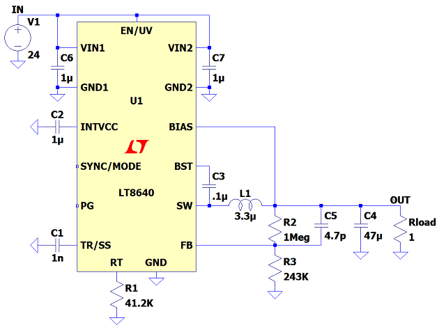
4. Advanced Evaluation: The LT8640 Regulator
The final section covers the simulation of a synchronous step-down regulator, specifically the Analog Devices LT8640.
LT8640 Regulator circuit in LTspice
Average vs. Switching Models
A critical distinction in this example is the use of simulation models:
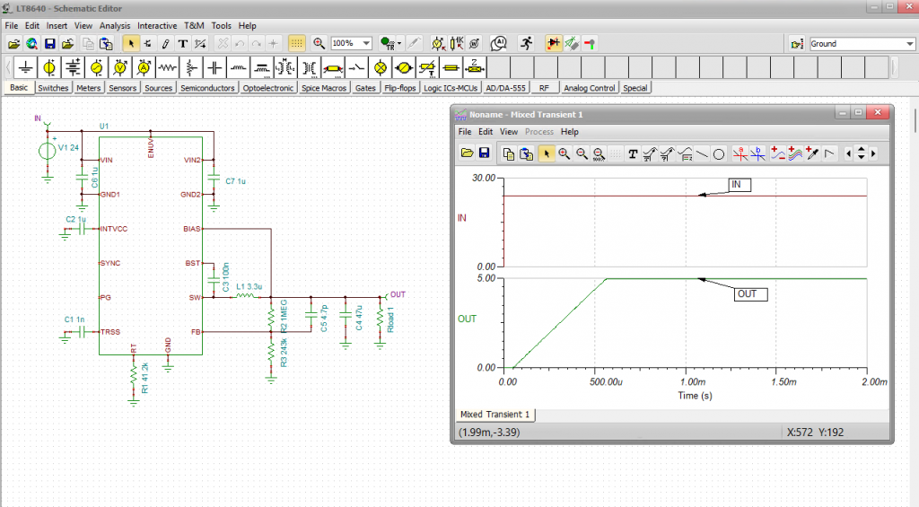
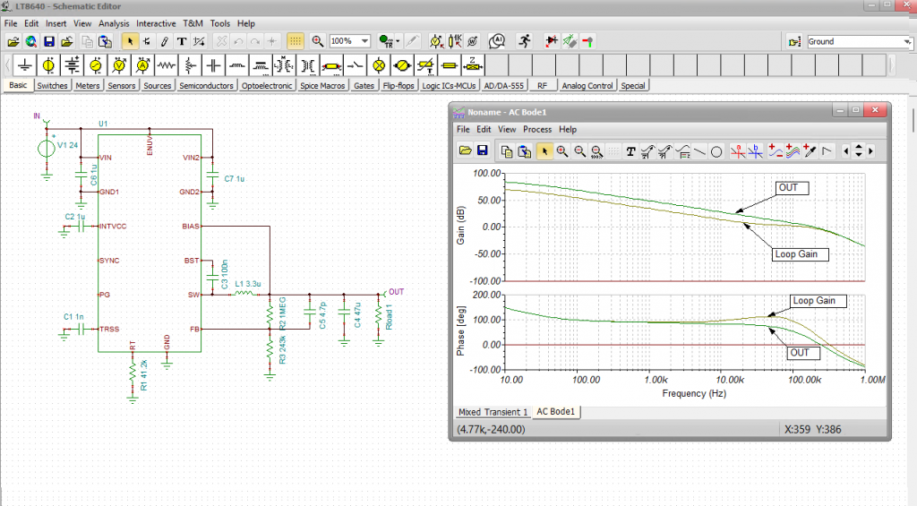
Average Models: These are utilized for exceptionally fast execution in the web browser and allow for AC frequency sweeps on the regulator’s control loop, which is vital for evaluating stability.
Switching Models: These provide high-fidelity time-domain simulations, but at the cost of longer execution times.
The LT8640 model used in TINA is an equivalent SPICE model independently developed by DesignSoft, based on manufacturer datasheets. This model follows standard SPICE conventions, making it compatible with other major simulators as well.
Presentation and Customization
To make simulation data more interpretable, the tutorial highlights several layout customization options:
Text Labels: Adding labels directly to curves for quick identification.
Separate Curves: Using this function to isolate signals into stacked diagrams, which helps in identifying phase and gain margins when viewing frequency responses like Loop Gain.
Transient analysis of the LT8640 regulator circuit in TINA, featuring detailed waveform labeling
AC Bode diagram for the LT8640 regulator in TINA, featuring labeled gain and phase curves
By following these procedures, engineers can ensure that designs migrated from LTspice are fully functional, verifiable, and well-documented within the TINA and TINACloud environments.