
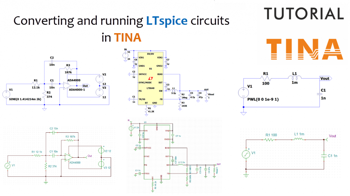
This post explores the workflow for migrating LTspice circuits (.asc files) into TINA, DesignSoft’s circuit simulator. We demonstrate how to import, execute, and evaluate these schematics locally on a computer. A key takeaway is the full cross-compatibility of the resulting .TSC files, which ensures a unified workflow between the TINA desktop application and the TINACloud platform.
Click here or on the image above to watch this blog presented as a video tutorial.
1. Importing and Basic Analysis (RLC Circuit Example)
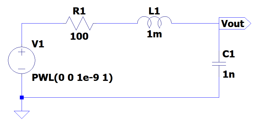
The conversion process is straightforward. By using the File > Import > LTspice command, users can bring LTspice designs into the TINA schematic editor. The tutorial demonstrates this using an educational RLC circuit.
Transient Analysis
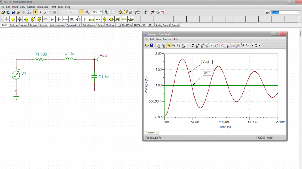
Once the schematic is imported, users can perform a Transient Analysis to examine the circuit in the time domain.
- Visualization: Waveforms are displayed in a diagram window.
- Customization: The “Collect Curves” function allows users to plot multiple signals (e.g., input and output) on the same coordinate system.
- Identification: The “Auto-Label Curves” tool helps identify voltages and currents directly on the graph.
AC Analysis
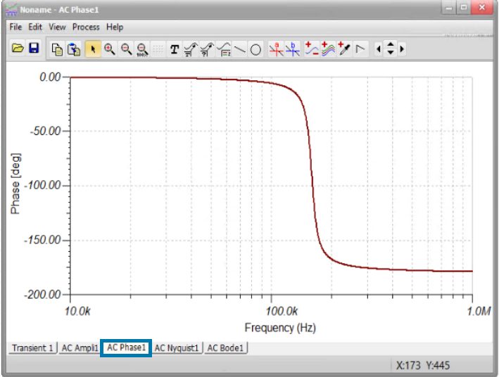
To explore frequency-domain behavior, the AC Transfer Characteristic is used. Beyond standard Bode plots, TINA provides:
- Multi-Diagram Output: Users can generate Amplitude, Phase, Nyquist, and Group Delay diagrams simultaneously.
- High-Resolution Results: By configuring start frequency and the number of plot points, users can generate detailed, high-resolution outputs across multiple tabs.
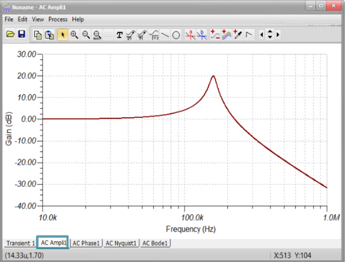
TINA AC analysis view: Amplitude diagram for the imported RLC circuit
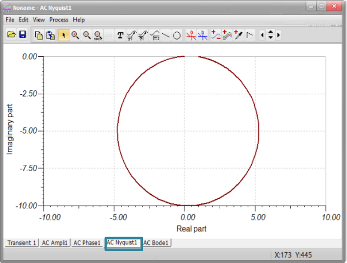
TINA AC analysis view: Nyquist diagram for the imported RLC circuit m
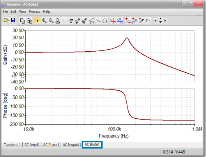
TINA AC analysis view: Bode diagram for the imported RLC circuit
2. Symbolic Analysis
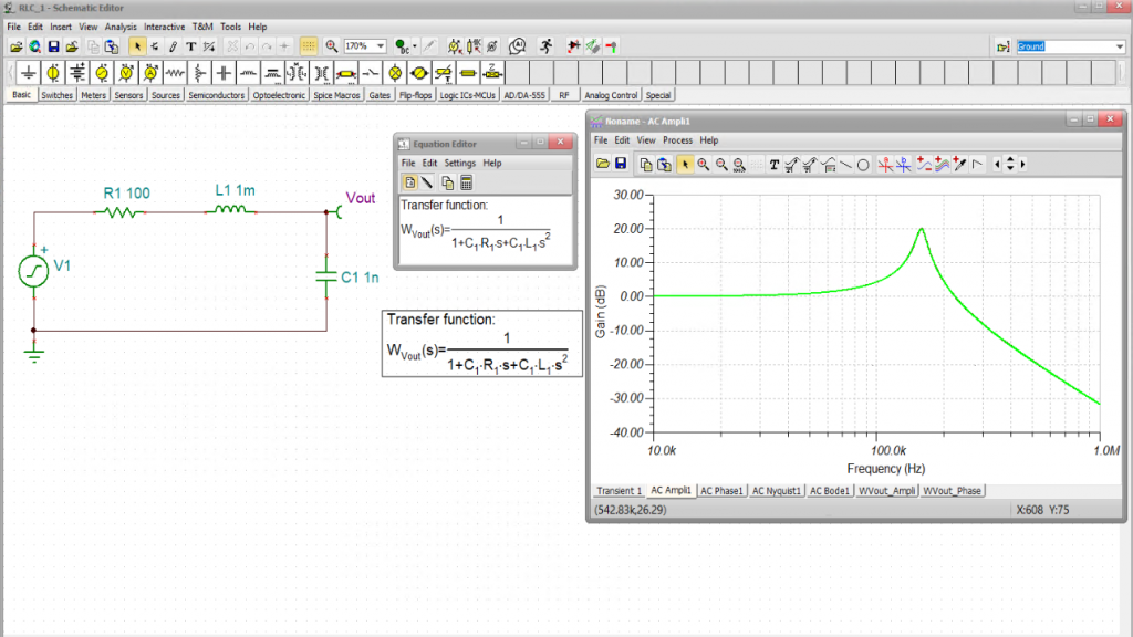
Another highlight of the tutorial is the ability to derive a circuit’s Transfer Function symbolically as an exact mathematical formula. This provides insights beyond numerical simulation, assisting in documentation and verification
Analytical Verification: The tutorial demonstrates how to extract this formula via the Equation Editor and paste it directly onto the schematic.
Curve Comparison: Users can plot the symbolic transfer function and overlay it on numerical simulation curves. A perfect alignment between the two confirms the circuit’s behavior and the accuracy of the model.
3. Active Filters and Operational Amplifiers
Using an active band-pass filter circuit based on the Analog Devices ADA4000-1 operational amplifier, the video shows how these analysis tools apply to standard building blocks.
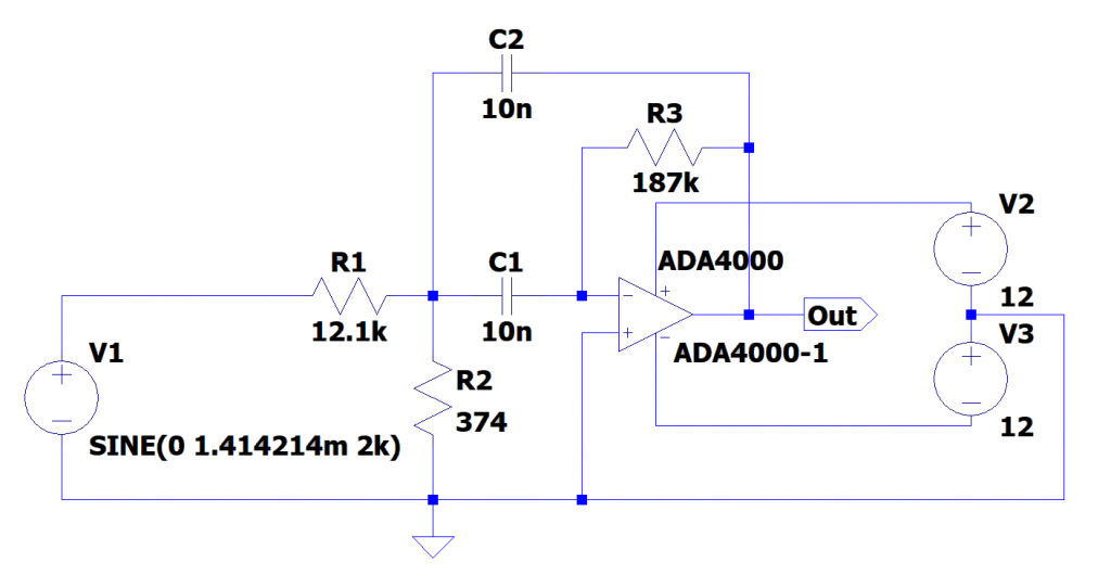
Active Band-pass filter (ADA4000-1) circuit in LTSpice
The workflow:
- Import the circuit file.
- Run AC Analysis to generate the combined Amplitude and Phase Bode Plot.
- Run Symbolic Analysis to derive the analytical transfer function.
- Overlay the analytical curves onto the numerical plots to verify that the results align.
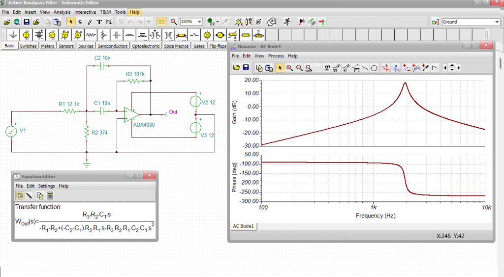
Active band-pass filter analysis in TINA, displaying the combined AC Bode plot and symbolic transfer function results
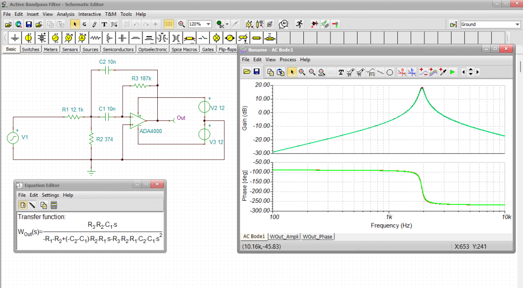
Active band-pass filter comparison: Overlaying analytical results onto numerical Bode plots
This also demonstrates that ideal operational amplifiers are well-suited for active filter synthesis, as the results consistently match the numerical simulations.
4. Advanced Evaluation: The LT8640 Regulator
The final section covers the simulation of a synchronous step-down regulator, specifically the Analog Devices LT8640.
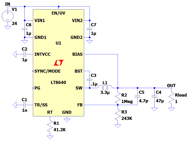
LT8640 Regulator circuit in LTspice
Average vs. Switching Models
A critical distinction in this example is the use of simulation models:
- Average Models: These are utilized for exceptionally fast execution in the web browser and allow for AC frequency sweeps on the regulator’s control loop, which is vital for evaluating stability.
- Switching Models: These provide high-fidelity time-domain simulations, but at the cost of longer execution times.
The LT8640 model used in TINA is an equivalent SPICE model independently developed by DesignSoft, based on manufacturer datasheets. This model follows standard SPICE conventions, making it compatible with other major simulators as well.
Presentation and Customization
To make simulation data more interpretable, the tutorial highlights several layout customization options:
- Text Labels: Adding labels directly to curves for quick identification.
- Separate Curves: Using this function to isolate signals into stacked diagrams, which helps in identifying phase and gain margins when viewing frequency responses like Loop Gain.
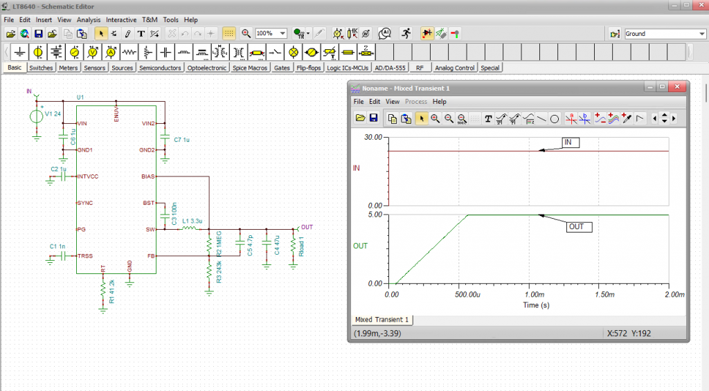
Transient analysis of the LT8640 regulator circuit in TINA, featuring detailed waveform labeling
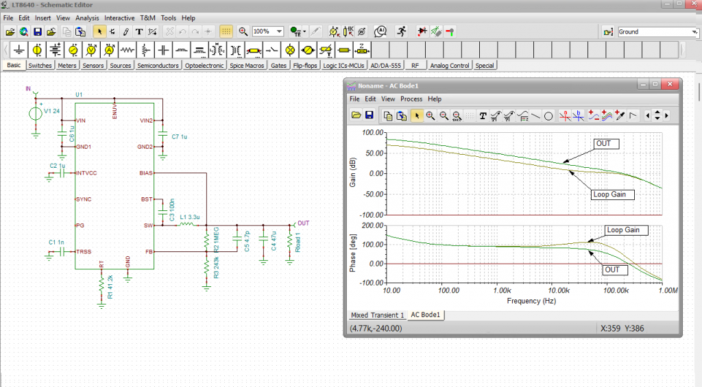
AC Bode diagram for the LT8640 regulator in TINA, featuring labeled gain and phase curves
By following these procedures, engineers can ensure that designs migrated from LTspice are fully functional, verifiable, and well-documented within the TINA and TINACloud environments.
- 📺 Watch the complete video tutorial: Watch on YouTube
- 🌐 Explore the software & features: Visit TINA Official Website