
12. Power Audio Op-amps
 CURRENT – 12. Power Audio Op-amps
 PREVIOUS- 11. Coupling between Multiple Inputs
Power Audio Op-amps
A common use for linear amplifiers is to provide gain for audio systems. An audio amplifier receives an input signal from a microphone, phonograph cartridge, tape deck, or AM/FM tuner. The output of the amplifier drives a speaker system, headphones, or a tape recorder. The input devices named above usually can be modeled by a voltage source with a low output voltage and high source impedance. Therefore the input impedance of the amplifier following this device must be high (much greater than the source impedance of the input device). In this manner, the amplifier does not significantly load the input device and the gain is not decreased.
The devices that are driven by the amplifier usually have low impedance. For example, the impedance of a single speaker is normally 8 Ω. These devices may require powers on the order of 1 to 10 W.
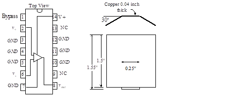
Figure 48 – The LM380 audio chip and optional heat sink
A variety of integrated circuit audio power op-amps, with different output powers, are available to the electronic design engineer. As an example, we present the LM380 audio power amplifier[1] which is used in such consumer applications as phono and tape deck amplifiers, intercoms, line drivers, alarms, TV sound systems, AM/FM radios, small servo drivers, and power converters. It has an internally fixed gain of 50 (34 dB) and an output that centers itself around one half of the supply voltage. Inputs can be either referenced to ground or balanced. The output stage is protected with both short circuit current limiting and thermal shutdown circuitry. The amplifier is packaged in a 14-pin DIP package as shown in Figure 48(a).
The output current is rated at 1.3 A peak. Since the device shuts down at junction temperatures above 150 oC, a heat sink [See Figure 48(b)] should be soldered to the unit. Maximum output power (with a heat sink) is 3.7 watts. The device is internally biased.
1The data and circuits are printed with the permission of the manufacturer, National Semiconductor Corp. The student is urged to use the data books when designing equipment with power op-amps.
Figure 49 shows the circuit configuration of a complete phono amplifier. A volume and tone control has been included in this circuit.
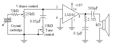
Figure 49 – Phono amplifier using LM380
12.1 Operational Amplifier Equivalent Circuit
If a particular application requires more power than can be obtained from a single power op-amp, we can use the bridge configuration of Figure 50.
Since this system provides twice the voltage swing across the load as the single-device system, the power capability is theoretically increased by a factor of 4 over the single amplifier (for a given power supply voltage). Since heat dissipation is the limiting concern in this design, we usually design the system conservatively and only double the output power.
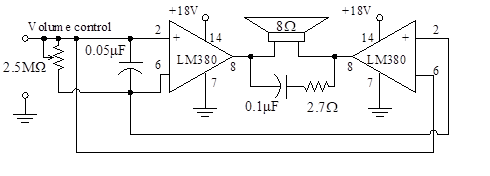
Figure 50 – Bridge configuration for high power
12.2 Intercom
Figure 51 shows an intercom incorporating a power op-amp and a few external components.
With the dual two-position switch (S1A-S1B) in the talk position (as shown in the figure), the speaker of the master station performs the function of a microphone, driving the power op-amp through a step-up transformer. The remote speaker is driven from the output of the power op-amp.
Switching S1A-S1B to the listen position reverses the role of master and remote. Now the remote speaker plays the role of the microphone, and it drives the power amplifier through a step-up transformer. The master speaker is now driven from the output of the power op-amp. The student should trace the wiring with S1A-S1B in the listen position to verify this. A step-up transformer with a turns ratio of 1:25 can be used, and the potentiometer, Rv, acts as the volume control.
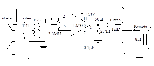
Figure 51 – Intercom
SUMMARY
This chapter built on the material presented in Chapter “Ideal Operational Amplifiers”, where we focused on the ideal operational amplifier. Although this important building block behaves almost as ideal amplifier, the design engineer must understand the contrasts between the practical device and the ideal model.
We began the chapter by examining the differential amplifier. We looked at the various configurations and transfer characteristics. Then we examined the typical operational amplifier, including packaging and internal circuitry. We looked at the manner in which the manufacturer specifies parameters for the amplifier.
Characteristics of practical op-amps were then presented, including gain, offset voltage, bias current, common-mode rejection, and power supply rejected ratio. Computer simulation models were next considered, followed by a detailed analysis of non-inverting and inverting amplifiers.
The chapter concluded with a variety of design considerations and examples. We examined balanced inputs and outputs and coupling between inputs. We also looked at power audio op-amps, including an example of an intercom circuit.
————
1The data and circuits are printed with the permission of the manufacturer, National Semiconductor Corp. The student is urged to use the data books when designing equipment with power op-amps.