
1. Ideal op-amps
 CURRENT – 1. Ideal op-amps
 PREVIOUS- Ideal Operational Amplifiers Introduction
Ideal op-amps
This section uses a systems approach to present the fundamentals of Ideal Operational Amplifiers. As such, we consider the op-amp as a block with input and output terminals. We are not currently concerned with the individual electronic devices within the op-amp.
An op-amp is an amplifier that is often powered by both positive and negative supply voltages. This allows the output voltage to swing both above and below ground potential. The op-amp finds wide application in many linear electronic systems.
The name operational amplifier is derived from one of the original uses of op-amp circuits; to perform mathematical operations in analog computers. This traditional application is discussed later in this chapter. Early op-amps used a single inverting input. A positive voltage change at the input caused a negative change at the output.
Hence, to understand the operation of the op-amp, it is necessary to first become familiar with the concept of controlled (dependent) sources since they form the basis of the op-amp model.
1.1 Dependent Sources
Dependent (or controlled) sources produce a voltage or current whose value is determined by a voltage or current existing in another location in the circuit. In contrast, passive devices produce a voltage or current whose value is determined by a voltage or current existing at the same location in the circuit. Both independent and dependent voltage and current sources are active elements. That is, they are capable of delivering power to some external device. Passive elements are not capable of generating power, although they can store energy for delivery at a later time, as is the case with capacitors and inductors.
The figure below illustrates an equivalent circuit configuration of an amplifying device often used in circuit analysis. The rightmost![]() resistor is the load. We will find the voltage and current gain of this system. Voltage gain, Av is defined as the ratio of output voltage to input voltage. Similarly, current gain, Ai is the ratio of output current to input current.
resistor is the load. We will find the voltage and current gain of this system. Voltage gain, Av is defined as the ratio of output voltage to input voltage. Similarly, current gain, Ai is the ratio of output current to input current.
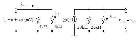
Figure 1- Equivalent circuit of a solid-state amplifying device
The input current is:
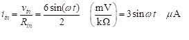
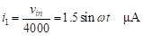
The current in the second resistor, i1, is found directly from Ohm’s law:
(2)
The output voltage is then given by:
(3)
In Equation (3), ‖ indicates a parallel combination of resistors. The output current is found directly from Ohm’s law.
(4)
The voltage and current gains are then found by forming the ratios:
(5)
(6)
1.2 Operational Amplifier Equivalent Circuit
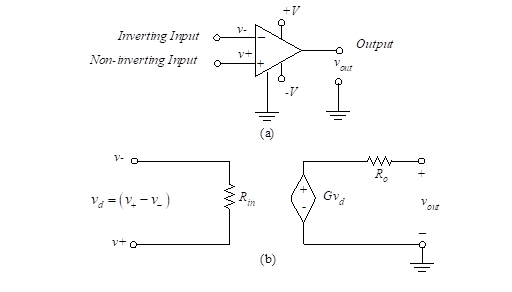
Figure 2- Operational amplifier and equivalent circuit
Figure 2 (a) presents the symbol for the operational amplifier, and Figure 2 (b) shows its equivalent circuit. The input terminals are v+ and v–. The output terminal is vout. The power supply connections are at the +V, -V and ground terminals. The power supply connections are often omitted from schematic drawings. The value of the output voltage is bounded by +V and -V since these are the most positive and negative voltages in the circuit.
The model contains a dependent voltage source whose voltage depends on the input voltage difference between v+ and v–. The two input terminals are known as the non-inverting and inverting inputs respectively. Ideally, the output of the amplifier does not depend on the magnitudes of the two input voltages, but only on the difference between them. We define the differential input voltage, vd, as the difference,
(7)
The output voltage is proportional to the differential input voltage, and we designate the ratio as the open-loop gain, G. Thus, the output voltage is
(8)
As an example, an input of ![]() (E is usually a small amplitude) applied to the non-inverting input with the inverting terminal grounded, produces
(E is usually a small amplitude) applied to the non-inverting input with the inverting terminal grounded, produces ![]() at the output. When the same source signal is applied to the inverting input with the non-inverting terminal grounded, the output is
at the output. When the same source signal is applied to the inverting input with the non-inverting terminal grounded, the output is ![]() .
.
The input impedance of the op-amp is shown as a resistance in Figure 2(b).
The output impedance is represented in the figure as a resistance, Ro.
An ideal operational amplifier is characterized as follows:
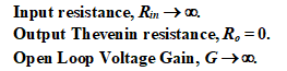
These are usually good approximations to the parameters of real op-amps. Typical parameters of real op-amps are:
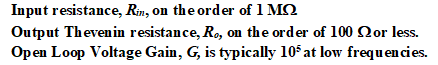
Using ideal op-amps to approximate real op-amps is therefore a valuable simplification for circuit analysis.
Let us explore the implication of the open-loop gain being infinite. If we rewrite Equation (8) ![]() as follows:
as follows:
(9)
and let G approach infinity, we see that
(10)
Equation (10) results by observing that the output voltage cannot be infinite. The value of the output voltage is bounded by the positive and negative power supply values. Equation (10) indicates that the voltages at the two terminals are the same:
(11)
Therefore, the equality of Equation (11) leads us to say there is a virtual short circuit between the input terminals.
Since the input resistance of the ideal op-amp is infinite, the current into each input, inverting terminal and non-inverting terminal, is zero.
When real op-amps are used in a linear amplification mode, the gain is very large, and Equation (11) is a good approximation. However, several applications for real op-amps use the device in a nonlinear mode. The approximation of Equation (11) is not valid for these circuits.
Although practical op-amps have high voltage gain, this gain varies with frequency. For this reason, an op-amp is not normally used in the form shown in Figure 2 (a). This configuration is known as open loop because there is no feedback from output to input. We see later that, while the open-loop configuration is useful for comparator applications, the more common configuration for linear applications is the closed-loop circuit with feedback.
External elements are used to “feedback” a portion of the output signal to the input. If the feedback elements are placed between the output and the inverting input, the closed-loop gain is decreased since a portion of the output subtracts from the input. We will see later that feedback not only decreases the overall gain, but it also makes that gain less sensitive to the value of G. With feedback, the closed-loop gain depends more on the feedback circuit elements, and less on the basic op-amp voltage gain, G. In fact, the closed-loop gain is essentially independent of the value of G-it depends only on values of the external circuit elements.
Figure (3) illustrates a single stage negative feedback op-amp circuit.
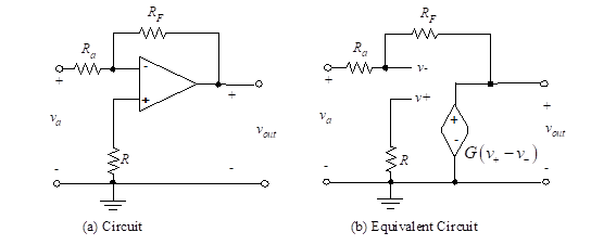
Figure 3- The inverting op-amp
Therefore, we will analyze this circuit in the next section. For now, note that a single resistor, RF, is used to connect the output voltage, vout to the inverting input, v–.
Another resistor, Ra is connected from the inverting input, v–, to the input voltage, va. A third resistor, R is placed between the non-inverting input and ground.
Circuits using op-amps, resistors and capacitors can be configured to perform many useful operations such as summing, subtracting, integrating, differentiating, filtering, comparing, and amplifying.
1.3 Analysis Method
We analyze circuits using the two important ideal op-amp properties:
- The voltage between v+ and v– is zero, or v+ = v–.
- The current into both the v+ and v– terminal is zero.
These simple observations lead to a procedure for analyzing any ideal op-amp circuit as follows:
- Write the Kirchhoff current law node equation at the non-inverting terminal, v+.
- Write the Kirchhoff current law node equation at the inverting terminal, v–.
- Set v+ = v– and solve for the desired closed-loop gains.
When applying Kirchhoff’s laws, remember that the current into both the v+ and v– terminal is zero.