Click or Tap the Example circuits below to invoke TINACloud and select the Interactive DC mode to Analyze them Online.
 Get a low cost access to TINACloud to edit the examples or create your own circuits
A sinusoidal voltage can be described by the equation:
v(t) = VM sin (ωt + Φ) or v(t) = VM cos (ωt + Φ)
| where | v(t) | Instantaneous value of the voltage, in volts (V). |
| VM | Maximum or peak value of the voltage, in volts (V) | |
| T | Period: The time taken for one cycle, in seconds | |
| f | Frequency – the number of periods in 1 second, in Hz (Hertz) or 1/s. f = 1/T | |
| ω | Angular frequency, expressed in radians/s ω = 2*π*f or ω = 2*π / T. | |
| Φ | Initial phase given in radians or degrees. This quantity determines the value of the sine or cosine wave att = 0. | |
| Note: The amplitude of a sinusoidal voltage is sometimes expressed as VEff, the effective or RMS value. This is related to VM according to the relationship VM=√2VEff, or approximately VEff = 0.707 VM |
Here are a few examples to illustrate the terms above.
The properties of the 220 V AC voltage in household electrical outlets in Europe:
Effective value: VEff = 220 V
Peak value: VM= √2*220 V = 311 V
Frequency: f = 50 1/s = 50 Hz
Angular frequency: ω = 2*π*f = 314 1/s = 314 rad/s
Period: T = 1/f = 20 ms
Time function: v(t)=311 sin (314 t)
Let’s see the time function using TINA’s Analysis/AC Analysis/Time Function command.
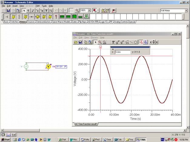
You can check that the period is T=20m and that VM = 311 V.
The properties of the 120 V AC voltage in the household electrical outlet in the US:
Effective value: VEff = 120 V
Peak value: VM=√2 120 V = 169.68 V ≈ 170 V
Frequency: f = 60 1/s = 60 Hz
Angular frequency: ω = 2*π*f= 376.8 rad/s ≈ 377 rad/s
Period: T = 1/f = 16.7 ms
Time function: v(t)=170 sin(377 t)
Note that in this case the time function could be given either as v(t)=311 sin (314 t+Φ) or v(t)=311 cos (314 t+Φ), since in the case of the outlet voltage we do not know the initial phase.
The initial phase plays an important role when several voltages are present simultaneously. A good practical example is the three-phase system, where three voltages of the same peak value, shape and frequency are present, each of which has a 120° phase shift relative to the others. In a 60 Hz network, the time functions are:
vA(t)=170 sin (377 t)
vB(t)=170 sin (377 t – 120°)
vC(t)=170 sin (377 t + 120°)
The following figure made with TINA shows the circuit with these time functions as TINA’s voltage generators.
The voltage difference vAB= vA(t) – vB(t) is shown as solved by TINA’s Analysis/AC Analysis/Time Function command.
Note that the peak of vAB (t) is approximately 294 V, larger than the 170 V peaksof the vA(t) or vB(t) voltages, but also not simply the sum of their peak voltages. This is due to the phase difference. We will discuss how to calculate the resulting voltage (which is Ö3 * 170 @ 294 in this case) later in this chapter and also in the separate Three-phase Systems chapter.
Characteristic values of sinusoidal signals
Though an AC signal continuously varies during its period, it is easy to define a few characteristic values for comparing one wave with another: These are the peak, average and root-mean-square (rms) values.
We have already met the peak value VM , which is simply the maximum value of the time function, the amplitude of the sinusoidal wave.
Sometimes the peak-to-peak (p-p) value is used. For sinusoidal voltages and currents, the peak-to-peak value is double the peak value.
The average value of the sine wave is the arithmetic average of the values for the positive half cycle. It is also called absolute average since it is the same as the average of the absolute value of the waveform. In practice, we encounter this waveform by rectifying the sine wave with a circuit called a full wave rectifier.
It can be shown that the absolute average of a sinusoidal wave is:
VAV= 2 / π VM ≅ 0.637 VM
Note that the average of a whole cycle is zero.
The rms or effective value of a sinusoidal voltage or current corresponds to the equivalent DC value producing the same heating power. For example, a voltage with an effective value of 120 V produces the same heating and lighting power in a light bulb as does 120 V from a DC voltage source. It can be shown that the rms or effective value of a sinusoidal wave is:

Vrms = VM / √2 ≅ 0.707 VM
These values can be calculated the same way for both voltages and currents.
The rms value is very important in practice. Unless indicated otherwise, power line AC voltages (e.g. 110V or 220V) are given in rms values. Most AC meters are calibrated in rms and indicate the rms level.
Example 1 Find the peak value of the sinusoidal voltage in an electrical network with 220 V rms value.
VM = 220/0.707 = 311.17 V
Example 2 Find the peak value of the sinusoidal voltage in an electrical network with 110 V rms value.
VM = 110/0.707 = 155.58 V
Example 3 Find the (absolute) average of the sinusoidal voltage if its rms value is 220 V.
Va = 0.637 * VM = 0.637*311.17 = 198.26 V
Example 4 Find the absolute average of the sinusoidal voltage if its rms value is 110 V.
The peak of the voltage from Example 2 is155.58 V and hence:
Va = 0.637 * VM = 0.637 * 155.58 = 99.13 V
Example 5 Find the ratio between the absolute average (Va) and rms (V) values for the sinusoidal waveform.
V/Va = 0.707/0.637 = 1.11
Note that you cannot add average values in an AC circuit because it leads to improper results.
PHASORS
As we have already seen in the previous section, it is often necessary in AC circuits to add sinusoidal voltages and currents of the same frequency. Though it is possible to add the signals numerically using TINA, or by employing trigonometric relations, it is more convenient to use the so-called phasor method. A phasor is a complex number representing the amplitude and phase of a sinusoidal signal. It is important to note that the phasor does not represent the frequency, which must be the same for all phasors.
A phasor can be handled as a complex number or represented graphically as a planar arrow in the complex plane. The graphic representation is called a phasor diagram. Using phasor diagrams, you can add or subtract phasors in a complex plane by the triangle or parallelogram rule.
There are two forms of complex numbers: rectangular and polar.
The rectangular representation is in the forma + jb, where j = Ö-1 is the imaginary unit.
The polar representation is in the form Aej j , where A is the absolute value (amplitude) and f is the angle of the phasor from the positive real axis, in the counterclockwise direction.
We will use bold letters for complex quantities.
Now let’s see how to derive the corresponding phasor from a time function.
First, assume that all the voltages in the circuit are expressed in the form of cosine functions. (All voltages can be converted to that form.) Then the phasor corresponding to the voltage of v(t) = VM cos( w t+f) is: VM = VMe jf , which is also called the complex peak value.
For example, consider the voltage: v(t) = 10 cos( w t+30°)
The corresponding phasor is:  V
V
We can calculate the time function from a phasor in the same way. First we write the phasor in polar form e.g. VM = VMe jr and then the corresponding time function is
v(t)=VM (cos(wt+r).
For example, consider the phasor VM =10 – j20 V
Bringing it to polar form:

And hence the time function is: v(t) = 22.36 cos(wt – 63.5°) V
Phasors are often used to define the complex effective or rms value of the voltages and currents in AC circuits. Given v(t) = VMcos(wt+r)= 10cos(wt+30°)
Numerically:
v(t) = 10*cos (wt-30°)
The complex effective (rms) value: V = 0.707*10* e– j30° = 7.07 e– j30° = 6.13 – j 3.535
Vice versa: if the complex effective value of a voltage is:
V = – 10 + j 20 = 22.36 e j 116.5°
then the complex peak value: 
and the time function: v(t) = 31.63 cos ( wt + 116.5° ) V
A short justification of the above techniques is as follows. Given a time function
VM (cos( w t+r), let’s define the complex time function as:
v (t) =VM e jr e jwt = VMe jwt = VM (cos(r) + j sin(r))e jwt
where VM =VM e j r t = VM (cos(r) + j sin(r)) is just the phasor introduced above.
For example, the complex time function of v(t)=10 cos(wt+30°)
v (t) = VMe jwt = 10 e j30 e jwt = 10e jwt (cos(30) + j sin(30))= e jwt (8.66+j5)
By introducing the complex time function, we have a representation with both a real part and an imaginary part. We can always recover the original real function of time by taking the real part of our result: v(t) = Re {v(t)}
However the complex time function has the great advantage that, since all the complex time functions in the AC circuits under consideration have the same ejwt multiplier, we can factor this out and just work with the phasors. Moreover, in practice we do not use the ejwt part at all–just the transformations from the time functions to the phasors and back.
To demonstrate the advantage of using phasors, let’s see the following example.
Example 6 Find the sum and the difference of the voltages:
v1 = 100 cos (314*t) and v2 = 50 cos (314*t-45°)
First write the phasors of both voltages:
V1M = 100 V2M= 50 e – j 45° = 35.53 – j 35.35
Hence:
Vadd = V1M + V2M = 135.35 – j 35.35 = 139.89 e– j 14.63°
Vsub = V1M – V2M = 64.65 + j35.35 = 73.68 e j 28.67°
and then the time functions:
vadd(t) = 139.89 * cos(wt – 14.63°)
vsub(t) = 73.68 * cos(wt + 28.67°)
As this simple example shows, the method of phasors.is an extremely powerful tool for solving AC problems.
Let’s solve the problem using the tools in TINA’s interpreter.
{calculation of v1+v2}
v1:=100
v2:=50*exp(-pi/4*j)
v2=[35.3553-35.3553*j]
v1add:=v1+v2
v1add=[135.3553-35.3553*j]
abs(v1add)=[139.8966]
radtodeg(arc(v1add))=[-14.6388]
{calculation of v1-v2}
v1sub:=v1-v2
v1sub=[64.6447+35.3553*j]
abs(v1sub)=[73.6813]
radtodeg(arc(v1sub))=[28.6751]
#calculation of v1+v2
import math as m
import cmath as c
v1=100
v2=50*c.exp(complex(0,-c.pi/4))
print(“v2=”,v2)
vadd=v1+v2
print(“vadd=”,vadd)
print(“abs(vadd)=”,abs(vadd))
print(“degrees(arc(vadd))=”,m.degrees(c.phase(vadd)))
#calculation of v1-v2
vsub=v1-v2
print(“vsub=”,vsub)
print(“abs(vsub)=”,abs(vsub))
print(“degrees(arc(vsub))=”,m.degrees(c.phase(vsub)))
The amplitude and phase results confirm the hand calculations.
Now lets check the result using TINA’s AC analysis.
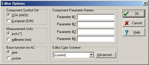
Before performing the analysis, let’s make sure that the Base function for AC ia set to cosine in the Editor Options dialog box from the View/Option menu. We will explain the role of this parameter at Example 8.
The circuits and the results:

Again the result is the same. Here are the time function graphs:
Example 7 Find the sum and the difference of the voltages:
v1 = 100 sin (314*t) and v2 = 50 cos (314*t-45°)
This example brings up a new question. So far we have required that all time functions be given as cosine functions. What shall we do with a time function given as a sine? The solution is to transform the sine function to a cosine function. Using the trigonometric relation sin(x)=cos(x-p/2)=cos(x-90°), our example can be rephrased as follows:
v1 = 100 cos(314t – 90°) and v2 = 50 cos (314*t – 45°)
Now the phasors of the voltages are:
V1M = 100 e – j 90° = -100 j V2M= 50 e – j 45° = 35.53 – j 35.35
Hence:
V add = V1M + V2M = 35.53 – j 135.35
V sub = V1M – V2M = – 35.53 – j 64.47
and then the time functions:
vadd(t) = 139.8966 cos(wt-75.36°)
vsub(t) = 73.68 cos(wt-118.68°)
Let’s solve the problem using the tools in TINA’s interpreter.