 Click or Tap the Example circuits below to invoke TINACloud and select the Interactive DC mode to Analyze them Online.
 Get a low cost access to TINACloud to edit the examples or create your own circuits
Most of the interesting functions of AC circuits –complex impedance, voltage transfer function, and current transfer ratio– depend on frequency. The dependence of a complex quantity upon frequency can be represented on a complex plane (Nyquist diagram) or on real planes as separate plots of the absolute value (amplitude plot) and the phase (phase plot).
Bode plots use a linear vertical scale for the amplitude plot, but since dB units are used, the effect is that the vertical scale is plotted according to the logarithm of the amplitude. The amplitude A is presented as 20log10(A). The horizontal scale for frequency is logarithmic.
Today, few engineers draw Bode plots by hand, relying instead on computers. TINA has very advanced facilities for Bode plots. Nevertheless, understanding the rules for drawing Bode plots will enhance your mastery of circuits. In the paragraphs that follow, we will present these rules and compare sketched straight-line approximation curves with TINA’s exact curves.
The function to be sketched is generally a fraction or a ratio with a numerator polynomial and a denominator polynomial. The first step is to find the roots of the polynomials. The roots of the numerator are the zeros of the function while the roots of the denominator are the poles.
Idealized Bode plots are simplified plots made up of straight-line segments. The end points of these straight-line segments projected onto the frequency axis fall on the pole and zero frequencies. The poles are sometimes called the cutoff frequencies of the network. For simpler expressions, we substitute s for frequency: jw = s.
Because the quantities being plotted are plotted on a logarithmic scale, the curves belonging to the different terms of the product can be added.
Here’s a summary of the important principles of Bode plots, and the rules for sketching them.
The 3 dB point on a Bode plot is special, representing the frequency at which the amplitude has increased from a constant value by 3 dB. Converting from A in dB to A in volts/volt, we solve 3 dB = 20 log10 A and obtain log10 A = 3/20 and hence  . The –3 dB point implies that A is 1/1.41 = 0.7.
A typical transfer function looks like this:
or
Now we will see how transfer functions like the ones above can be quickly sketched (transfer function gain in dB versus frequency in Hz). Because the vertical axis is represented in dB, it is a logarithmic scale. Remembering that the product of terms in the transfer function will be seen as the sum of terms in the logarithmic domain, we will see how to sketch the individual terms separately and then add them graphically to obtain the final result.
The curve of the absolute value of a first order term s has a 20 dB/decade slope crossing the horizontal axis at w = 1. The phase of this term is 90° at any frequency. The curve of K*s also has a 20 dB/decade slope but it crosses the axis at w = 1/K; i.e., where the absolute value of the product ½K*s ½= 1.
The next first order term (in the second example), s-1 = 1/s, is similar: its absolute value has a -20 dB/decade slope; its phase is -90° at any frequency; and it crosses the w-axis at w = 1. Similarly, the absolute value of the term K/s has a -20 dB/decade slope; the phase is -90° at any frequency; but it crosses the w axis at w = K, where the absolute value of the fraction
½K/s ½= 1.
The next first order term to sketch is 1+sT. The amplitude plot is a horizontal line until w1 = 1/T, after which it slopes upward at 20 dB/decade. The phase equals zero at small frequencies, 90° at high frequencies and 45° at w1 = 1/T. A good approximation for phase is that it is zero until 0.1*w1 = 0.1/T and is nearly 90° above 10*w1 = 10/T. Between these frequencies, the phase diagram can be approximated by a straight-line segment which connects the points (0.1*w1; 0) and (10*w1; 90°).
The last first order term, 1/(1+sT), has a –20 dB/decade slope starting at the angular frequency w1=1/T. The phase is 0 at small frequencies, -90° at high frequencies, and -45° at w1 = 1/T. Between these frequencies, the phase diagram can be approximated by a straight line which connects the points (0.1*w1; 0) and (10*w1; – 90°).
A constant multiplier factor in the function is plotted as a horizontal line parallel to w-axis.
Second order polynomials with complex conjugate roots lead to a more complicated Bode plot that will not be considered here.
Example 1
Find the equivalent impedance and sketch it.
You can use TINA Analysis to get the equation of the equivalent impedance by choosing Analysis – Symbolic analysis – AC Transfer.
The total impedance: Z(s) = R + sL = R (1 + sL/R)
…and the cutoff frequency: w1 = R/L = 5/0.5 = 10 rad/s f1 = 1.5916 Hz
The cutoff frequency can be seen as the +3 dB point in the Bode plot. Here the 3 dB point means 1.4*R = 7.07 ohm. |
You can also have TINA plot the amplitude and phase characteristics each on its own graph:
|
|
Note that the plot of impedance uses a linear vertical scale, not logarithmic, so we cannot use the 20 dB/decade tangent. In both the impedance and phase plots, the x-axis is the w axis scaled for frequency in Hz. For the impedance diagram, the y-axis is linear and displays impedance in ohms. For the phase diagram, the y-axis is linear and displays phase in degrees.
Example 2
Find the transfer function for VC/VS. Sketch the Bode plot of this function.
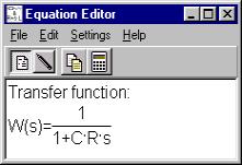
We obtain the transfer function using voltage division:
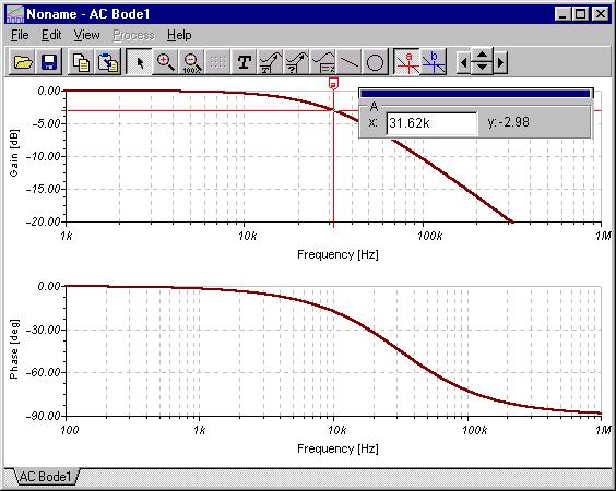
The cutoff frequency: w1 = 1/RC = 1/5*10-6 = 200 krad/s f1 = 31.83 kHz
One of TINA’s strong features is its symbolic analysis: Analysis – ‘Symbolic Analysis’ – AC transfer or Semi-Symbolic AC transfer. These analyses give you the transfer function of the network either in full symbolic form or in semi-symbolic form. In semi-symbolic form, the numerical values for component values are used and the only remaining variable is s.
TINA draws the actual Bode plot, not a straight-line approximation. To find the actual cutoff frequency, use the cursor to locate the–3 dB point.
 |
In this second plot, we used TINA’s annotation tools to draw the straight-line segments also.
|
Once again, the y-axis is linear and displays the voltage ratio in dB or the phase in degrees. The x- or w-axis represents frequency in Hz.
In the third example we illustrate how we obtain the solution by adding the different terms.
Example 3
Find the voltage transfer characteristic W = V2/VS and draw its Bode diagrams.
Find the frequency where the magnitude of W is minimum.
Obtain the frequency where the phase angle is 0.
The transfer function can be found using ‘Symbolic analysis’ ‘AC transfer” in TINA’s analysis menu.
 |
Or with ‘Semi-symbolic AC transfer’.
 |
Manually, using Mohm, nF, kHz units:
First find the roots:
the zeros w01 = 1/(R1C1) = 103 rad/s and w02 = 1/(R2C2) = 2*103 rad/s
f01 = 159.16 Hz and f02 = 318.32 Hz
and poles wP1 = 155.71 rad/s and wP2 = 12.84 krad/s
fP1 = 24.78 Hz and fP2 = 2.044 kHz
The transfer function in a so called ‘normal form’:
The second normalized form is more convenient for drawing the Bode plot.
First, find the transfer function value at f = 0 (DC). By inspection, it is 1, or 0dB. This is the starting value of our straight-line approximation of W(s). Draw a horizontal line segment from DC to the first pole or zero, at the 0dB level.
Next, order the poles and zeroes by ascending frequency:
fP1 = 24.78 Hz
f01 =159.16 Hz
f02 = 318.32 Hz
fP2 = 2.044 kHz
Now at the first pole or zero (it happens to be a pole, fP1), draw a line, in this case falling at 20dB/decade.
At the next pole or zero, f01, draw a level line segment reflecting the combined effect of the pole and zero (their slopes cancel).
At f02, the second and last zero, draw a rising line segment (20dB/decade) to reflect the combined effect of the pole/zero/zero.
At fP2, the second and last pole, change the slope of the rising segment to a level line, reflecting the net effect of two zeroes and two poles.
The results are shown on the Bode plot of amplitude that follows, where the straight-line segments are shown as thin dash-dot-dot lines.
Next, we draw the thick lime line to summarize these segments.
Finally, we have TINA’s calculated Bode function plotted in maroon.
|
You can see that when a pole is very near a zero, the straight-line approximation deviates quite a bit from the actual function. Also note the minimum gain in the Bode plot above. With a somewhat complicated network such as this, it is difficult to find the minimum gain from the straight-line approximation, although the frequency at which the minimum gain occurs can be seen.
|
In the TINA Bode plots above, the cursor is used to find Amin and the frequency at which the phase passes through 0 degrees.
Amin @ -12.74 dB ® Amin = 0.23 at f = 227.7 Hz
and j = 0 at f = 223.4 Hz.