 Click or Tap the Example circuits below to invoke TINACloud and select the Interactive DC mode to Analyze them Online.
 Get a low cost access to TINACloud to edit the examples or create your own circuits
Circuits containing R, L, C elements often have special characteristics useful in many applications. Because their frequency characteristics (impedance, voltage, or current vs. frequency) may have a sharp maximum or minimum at certain frequencies these circuits are very important in the operation of television receivers, radio receivers, and transmitters. In this chapter we will present the different types, models and formulas of typical resonant circuits.
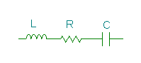
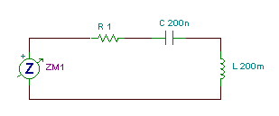
SERIES RESONANCEA typical series resonant circuit is shown in the figure below.
 The total impedance:
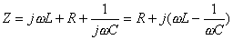
In many cases, R represents the loss resistance of the inductor, which in the case of air core coils simply means the resistance of the winding. The resistances associated with the capacitor are often negligible.
The impedances of the capacitor and inductor are imaginary and have opposite sign. At the frequency w0 L= 1/w0C, the total imaginary part is zero and therefore the total impedance is R, having a minimum at the w0frequency. This frequency is called the series resonant frequency.
The typical impedance characteristic of the circuit is shown in the figure below.
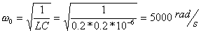
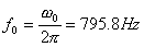
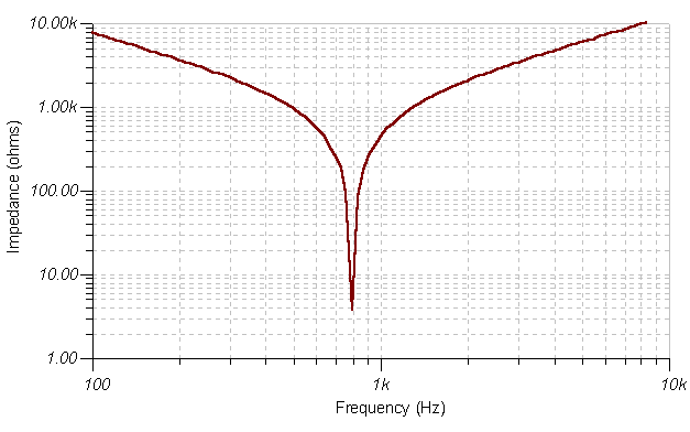 From the w0L= 1/w0Cequation, the angular frequency of the series resonance: or for the frequency in Hz:f0This is the so-called Thomson formula.If R is small compared to the XL, XC reactance around the resonant frequency, the impedance changes sharply at the series resonant frequencyIn this case we say that the circuit has good selectivity.The selectivity can be measured by the quality factor Q If the angular frequency in the formula equals the angular frequency of resonance, we get the resonant quality factor There is a more general definition of the quality factor:
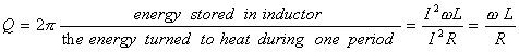 The voltage across the inductor or capacitor can be much higher then the voltage of the total circuit. At the resonant frequency the total impedance of the circuit is:
Z=R
Assuming that the current through the circuit is I, total voltage on the circuit is
Vtot=I*R
However the voltage on the inductor and the capacitor
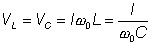
Therefore
This means at the resonant frequency the voltages on the inductor and the capacitor are Q0 times greater than the total voltage of the resonant circuit.
The typical run of the VL, VC voltages is shown in the figure below.

Let’s demonstrate this via a concrete example.
Example 1
Find the frequency of resonance (f0) and the resonant quality factor (Q0) in the series circuit below, if C=200nF, L=0.2H, R=200 ohms, and R=5 ohms. Draw the phasor diagram and the frequency response of the voltages.
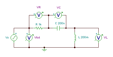

For R=200 ohms
This is a quite low value for practical resonant circuits, which normally have quality factors over 100. We have used a low value to more easily demonstrate the operation on a phasor diagram.
The current at the resonance frequency I=Vs/R=5m>
The voltages at current of 5mA: VR = Vs =1 V
meanwhile: VL = VC = I*w0L = 5*10-3 *5000*0.2 = 5V
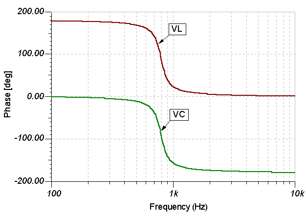
The ratio between VL, VC,and Vs is equal to the quality factor!Now let’s see the phasor diagram by calling it from the AC Analysis menu of TINA.
We used the Auto Label tool of the diagram window to annotate the picture.
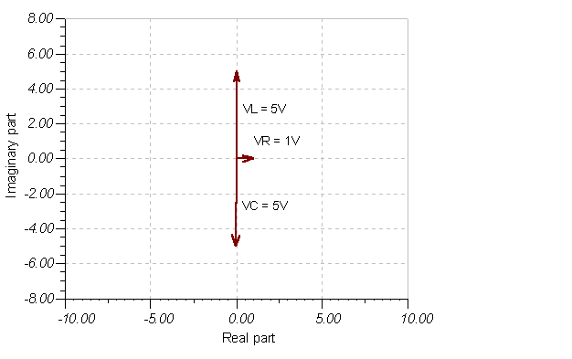
The phasor diagram nicely shows how the voltages of the capacitor and inductor cancel each other at the resonance frequency.
Now let’s see VLand VCversus frequency.
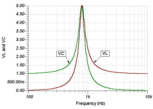
Note that VL starts from zero voltage (because its reactance is zero at zero frequency) while VC starts from 1 V (because its reactance is infinite at zero frequency). Similarly VL tends to 1V and VCto 0V at high frequencies.
Now for R=5 ohms the quality factor is much greater:
This is a relatively high quality factor, close to the practical achievable values.
The current at the resonance frequency I=Vs/R=0.2A
meanwhile: VL = VC = I*w0L = 0.2*5000*0.2 = 200
Again the ratio between the voltages equals the quality factor!
Now let’s draw just VL and VC voltages versus frequency. On the phasor diagram, VR would be too small compared to VLand VC
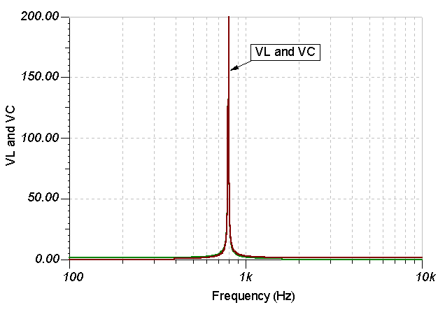
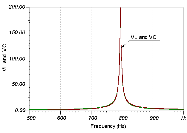
As we can see, the curve is very sharp and we needed to plot 10,000 points to get the maximum value accurately. Using a narrower bandwidth on the linear scale on the frequency axis, we get the more detailed curve below.
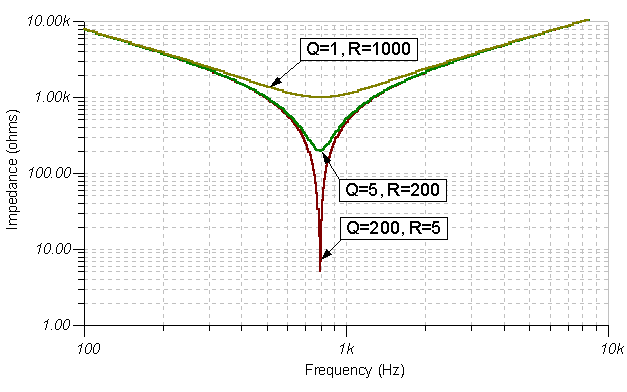
Finally let’s see the impedance characteristic of the circuit: for different quality factors.
The figure below was created using TINA by replacing the voltage generator by an impedance meter. Also, set up a parameter stepping list for R = 5, 200, and 1000 ohms. To set up parameter stepping, select Control Object from the Analysis menu, move the cursor (which has changed into a resistor symbol) to the resistor on the schematic, and click with the left mouse button. To set a logarithmic scale on the Impedance axis, we have double-clicked on the vertical axis and set Scale to Logarithmic and the limits to 1 and 10k.
PARALLE RESONANCE
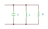
The pure parallel resonant circuit is shown in the figure below.
If we neglect the loss resistance of the inductor, R represents the leakage resistance of the capacitor. However, as we will see below the loss resistance of the inductor can be transformed into this resistor.
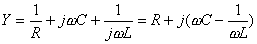
The total admittance:
The total impedance characteristic of the pure parallel resonant circuit is shown in the figure below:
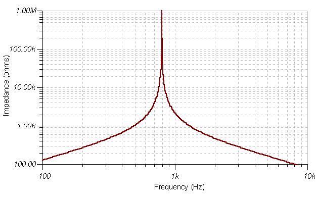
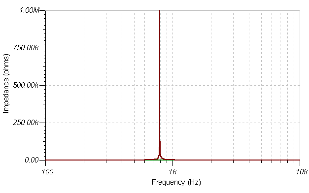
Note that the impedance changes very rapidly around the resonance frequency, even though we used a logarithmic impedance axis for better resolution. The same curve with a linear impedance axis is shown below. Note that viewed with this axis, the impedance appears to be changing even more rapidly near resonance.
The susceptances of the inductance and capacitance are equal but of opposite sign at resonance: BL = BC, 1/w0L = w0C, hence the angular frequency of the parallel resonance:

determined again by the Thomson formula.
Solving for the resonant frequency in Hz:

At this frequency the admittance Y = 1/R = G and is at its minimum (i.e., the impedance is maximum). The currents through the inductance and capacitance can be much higher then the current of the total circuit. If R is relatively large, the voltage and admittance changes sharply around the resonant frequency. In this case we say the circuit has good selectivity.
Selectivity can be measured by the quality factor Q
When the angular frequency equals the angular frequency of resonance, we get the resonant quality factor
There is also a more general definition of the quality factor:

Another important property of the parallel resonant circuit is its bandwidth. The bandwidth is the difference between the two cutoff frequencies, where the impedance drops from its maximum value to 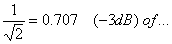 the maximum.
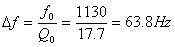
It can be shown that the Δf bandwidth is determined by the following simple formula:

This formula is also applicable for series resonant circuits.
Let us demonstrate the theory through some examples.
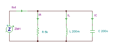
Example 2
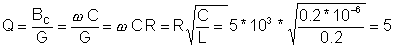
Find the resonant frequency and the resonant quality factor of a pure parallel resonance circuit where R = 5 kohm, L = 0.2 H, C = 200 nF.
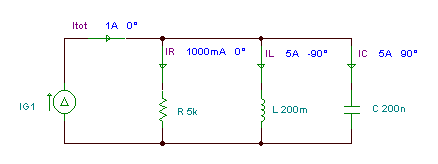
The resonant frequency:
and the resonant quality factor:
Incidentally, this quality factor is equal to IL /IR at the resonant frequency.
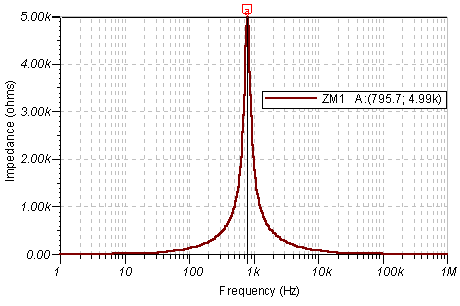
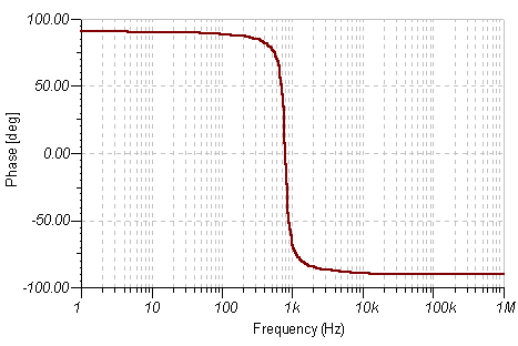
Now let us draw the impedance diagram of the circuit:
The simplest way is to replace the current source by an impedance meter and run an AC Transfer analysis.
 <
<
The “pure” parallel circuit above was very easy to examine since all components were in parallel. This is especially important when the circuit is connected to other parts.
However in this circuit, the series loss resistance of the coil was not considered.
Now let’s examine the following so called “real parallel resonant circuit,” with the series loss resistance of the coil present and learn how we can transform it into a “pure” parallel circuit.
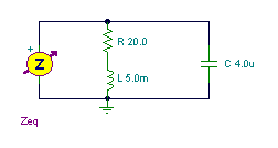
The equivalent impedance:
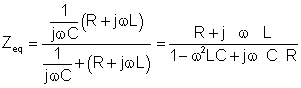
Let’s examine this impedance at the resonant frequency where 1-w02LC=0
We will also assume that the quality factor Qo = woL/ RL>>1.
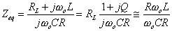
At the resonant frequency
Since at resonant frequencyw0L= 1/w0C
Zeq=Qo2 RL
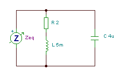
Since in the pure parallel resonant circuit at the resonant frequency Zeq = R, the real parallel resonant circuit can be replaced by a pure parallel resonant circuit, where:
R = Qo2 RL
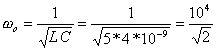
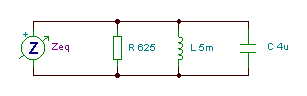
Example 3
Compare the impedance diagrams of a real parallel and its equivalent pure parallel resonance circuit.
The resonant (Thomson) frequency:
The impedance diagram is the following:

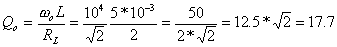
The equivalent parallel resistance: Req = Qo2 RL = 625 ohm
The equivalent parallel circuit:
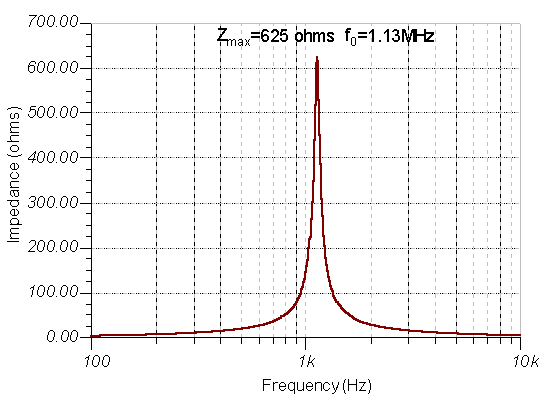
The impedance diagram:
Finally, if we use copy and paste to see both curves on one diagram, we get the following picture where the two curves coincide.
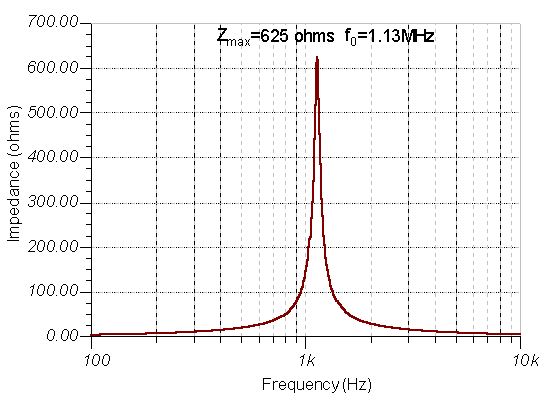
Finally let’s examine the bandwidth of this circuit.
The calculated value:
Lets confirm it graphically using the diagram.
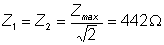
Zmax = 625 ohm. The impedance limits that define the cutoff frequencies are:
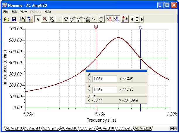
The difference of the A-B cursors is 63.44Hz, which is in very good agreement with the theoretical 63.8Hz result even taking the inaccuracy of the graphic procedure into consideration.