Click or Tap the Example circuits below to invoke TINACloud and select the Interactive DC mode to Analyze them Online.
Get a low cost access to TINACloud to edit the examples or create your own circuits

SUPERPOSITION IN AC CIRCUITS

KIRCHHOFF’S LAWS IN AC CIRCUITS

Thévenin’s Theorem for AC circuits with sinusoidal sources is very similar to the theorem we have learned for DC circuits. The only difference is that we must consider impedance instead of resistance. Concisely stated, Thévenin’s Theorem for AC circuits says:

Any two terminal linear circuit can be replaced by an equivalent circuit consisting of a voltage source (V_Th) and a series impedance (Z_Th).

In other words, Thévenin’s Theorem allows one to replace a complicated circuit with a simple equivalent circuit containing only a voltage source and a series connected impedance. The theorem is very important from both theoretical and practical viewpoints.

It is important to note that the Thévenin equivalent circuit provides equivalence at the terminals only. Obviously, the internal structure of the original circuit and the Thévenin equivalent may be quite different. And for AC circuits, where impedance is frequency dependent, the equivalence is valid at one frequency only.

Using Thévenin’s Theorem is especially advantageous when:

· we want to concentrate on a specific portion of a circuit. The rest of the circuit can be replaced by a simple Thévenin equivalent.

· we have to study the circuit with different load values at the terminals. Using the Thévenin equivalent we can avoid having to analyze the complex original circuit each time.

We can calculate the Thévenin equivalent circuit in two steps:

1. Calculate Z_Th. Set all sources to zero (replace voltage sources by short circuits and current sources by open circuits) and then find the total impedance between the two terminals.

2. Calculate V_Th. Find the open circuit voltage between the terminals.

Norton’s Theorem, already presented for DC circuits, can also be used in AC circuits. Norton’s Theorem applied to AC circuits states that the network can be replaced by a current source in parallel with an impedance.

We can calculate the Norton equivalent circuit in two steps:

1. Calculate Z_Th. Set all sources to zero (replace voltage sources by short circuits and current sources by open circuits) and then find the total impedance between the two terminals.

2. Calculate I_Th. Find the short circuit current between the terminals.

Now let’s see some simple examples.

Example 1

Find the Thévenin equivalent of the network for the points A and B at a frequency: f = 1 kHz, v_S(t) = 10 cosw×t V.

The first step is to find the open circuit voltage between points A and B:

The open circuit voltage using voltage division:

= -0.065 – j2.462 = 2.463 e^-j91.5º V

Checking with TINA:

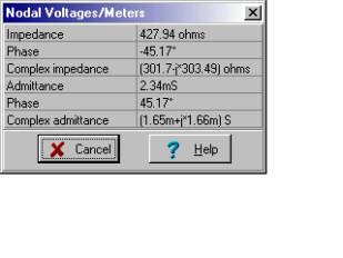
The second step is to replace the voltage source by a short circuit and to find the impedance between points A and B:

Here is the Thévenin equivalent circuit, valid only at a frequency of 1kHz. We must first, however, solve for CT’s capacitance. Using the relationship 1/wC_T = 304 ohm, we find C_T = 0.524 uF

Now we have the solution: R_T = 301 ohm and C_T = 0.524 m F:

Next, we can use TINA’s interpreter to check our calculations of the Thévenin equivalent circuit:

Note that in the listing above we used a function “replus.’ Replus solves for the parallel equivalent of two impedances; i.e., it finds the product over the sum of the two parallel impedances.

Example 2

Find the Norton equivalent of the circuit in Example 1.

f = 1 kHz, v_S(t) = 10 cosw×t V.

The equivalent impedance is the same:

Z_N=(0.301-j0.304) kW

Next, find the short-circuit current:

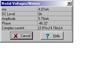
I_N = (3.97-j4.16) mA

And we can check our hand calculations against TINA’s results. First the open circuit impedance:

Then the short-circuit current:

And finally the Norton equivalent:

Next, we can use TINA’s interpreter to find the Norton equivalent circuit components:

Example 3

In this circuit, the load is the series-connected RL and CL. These load components are not part of the circuit whose equivalent we are seeking. Find the current in the load using the Norton equivalent of the circuit.

v₁(t) = 10 cos wt V; v₂(t) = 20 cos (wt+30°) V; v₃(t) = 30 cos (wt+70°) V;

v₄(t) = 15 cos (wt+45°) V; v₅(t) = 25 cos (wt+50°) V; f = 1 kHz.

First find the open circuit equivalent impedance Z_eq by hand (without the load).

Numerically

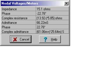
Z_N = Z_eq = (13.93 – j5.85) ohm.

Below we see TINA’s solution. Note that we replaced all the voltage sources with short circuits before we used the meter.

Now the short-circuit current:

The calculation of the short-circuit current is quite complicated. Hint: this would be a good time to use Superposition. An approach would be to find the load current (in rectangular form) for each voltage source taken one at a time. Then sum the five partial results to get the total.

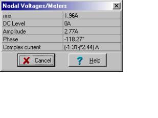
We will just use the value provided by TINA:

i_N(t) = 2.77 cos (w×t-118.27°) A

Putting it all together (replacing the network with its Norton equivalent, reconnecting the load components to the output, and inserting an ammeter in the load), we have the solution for the load current that we sought:

By hand calculation, we could find the load current using current division:

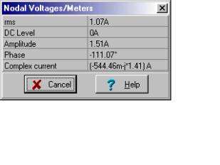
Finally

I = (- 0.544 – j 1.41) A

and the time function

SUPERPOSITION IN AC CIRCUITS

KIRCHHOFF’S LAWS IN AC CIRCUITS