SPICE, SPICE, SPICE when you do electronic circuit simulation you always hear these magic words. What is this and why is this so important? We will explain that in this free Internet course and teach you how to use, add and create sophisticated device models for your simulation software. In our material we will you the TINA and TINACloud software for demonstration of the circuits and models we will create, however our SPICE models and circuits work in most SPICE simulators without any changes.
Creating a SPICE model for a comparator with hysteresis
Creating a SPICE models for practical gate drivers
Adding SPICE models to TINA and TINACloud
.SUBCKT- Sub-circuit description
E – Voltage-Controlled Voltage Source, G – Voltage-Controlled Current Source
F – Current-Controlled Current Source, H – Current-Controlled Voltage Source
I – Independent Current Source, V – Independent Voltage Source
K – Inductor Coupling (Transformer Core)
SOURCES – Transient Source Descriptions
FUNCTIONS – Functions in Expression
Spice simulation is a circuit simulation method developed at the University of California, Berkeley, first presented in 1973. The last 3f5 version of Berkeley Spice was released in 1993. Berkely Spice serves as a basis for most circuit simulation programs in academia and in the industry. Today’s Spice simulators are of course more advanced and sophisticated than the original Berkely Spice simulator and are extended in many ways. One huge advantage of Spice simulation, that semiconductor manufacturers provide large free libraries for their products using Spice models, which most Spice simulators can open and use.
Creating a SPICE model for a comparator with hysteresis
Creating a SPICE models for practical gate drivers
Adding SPICE models to TINA and TINACloud
![]() Creating Subcircuits from Spice Models in TINA: .MODEL format
Creating Subcircuits from Spice Models in TINA: .MODEL format
![]() Creating Subcircuits from Spice Netlists in TINA, part 1: Simple 5-terminal Operational Amplifiers
Creating Subcircuits from Spice Netlists in TINA, part 1: Simple 5-terminal Operational Amplifiers
![]() Creating Subcircuits from Spice Netlists in TINA, part 2: Complex multi-terminal Op Amps
Creating Subcircuits from Spice Netlists in TINA, part 2: Complex multi-terminal Op Amps
You can find more tutorials at
![]() Adding Spice, S-parameter and Schematic macros to TINA & TINACloud
Adding Spice, S-parameter and Schematic macros to TINA & TINACloud
General Format:
.MODEL <name> [AKO: <reference model name>] <type>
+ ([<parameter name> = <value> [tolerance specfication]]*)
The .MODEL statement describes a set of device parameters which are used in the net list for certain components. <name> is the model name which the components used. <type> is the device type and must be one of the following:
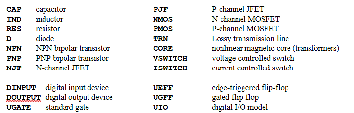
Following <type> is the list of parameters which describe the model for the device. None, any, or all parameters may be assigned values, those that are not assigned take on default values. The lists of parameter names, meanings, and default values are located in the individual device descriptions.
LT and SIMetrix using an A device for representing digital primitives.
Example:
.MODEL RMAX RES (R=1.5 TC1=0.0002 TC2=0.005)
.MODEL DNOM D (IS=1E-9)
.MODEL QDRIV NPN (IS=1E-7 BF=30)
.MODEL QDR2 AKO:QDRIV NPN (BF=50 IKF=50m)
General Formats:
.PARAM < <name> = <value> >*
.PARAM < <name> = { <expression> } >*
The .PARAM statement defines the value of a parameter. A parameter name can be used in place of most numeric values in the circuit description. Parameters can be constants, or expressions involving constants, or a combination of these, and they can include other parameters.
Predefined parameters: TEMP, VT, GMIN, TIME, S, PI, E
Example:
.PARAM VCC = 12V, VEE = -12V
.PARAM BANDWIDTH = {100kHz/3}
.PARAM PI = 3.14159, TWO_PI = {2*3.14159}
.PARAM VNUM = {2*TWO_PI}
.SUBCKT-Sub-circuit description
General Formats:
.SUBCKT <name> [node]*
+ [OPTIONAL: < <interface node> = <default value> >*]
+ [PARAMS: < <name> = <value> >* ]
.SUBCKT declares that a Sub-circuit of the net list will be described until the .ENDS command. Sub-circuits are called in the net list by the command, X. <name> is the Sub-circuits name. [node]* is an optional list of nodes local only to the Sub-circuit and used for connection on the top level. Sub-circuit calls can be nested (can have X inside). However, Sub-circuits cannot be nested (no .SUBCKT inside).
Example:
.SUBCKT OPAMP 1 2 101 102 17
…
.ENDS
.SUBCKT FILTER INPUT OUTPUT PARAMS: CENTER=100kHz,
+ BANDWIDTH=10kHz
…
.ENDS
.SUBCKT 74LS00 A B Y
+ OPTIONAL: DPWR=$G_DPWR DGND=$G_DGND
+ PARAMS: MNTYMXDLY=0 IO_LEVEL=0
…
.ENDS
General Formats:
C<name> <+ node> <- node> [model name] <value> [IC = <initial value>]
[model name] is optional and if not included then <value> is the capacitance in farads. If [model name] is specified then the capacitance is given by:
Ctot = |value| * C * [1+ TC1*(T-Tnom) + TC2 * (T-Tnom)2]
where C, TC1, and TC2 are described below. Ctot is the total capacitance. T is the simulation temperature. And Tnom is the nominal temperature (27°C unless set by in Analysis.Set Analysis dialog)
<value> can either be positive or negative.
[IC = <initial value>] gives PSPICE an initial guess for voltage across the capacitor during bias point calculation and is optional.
| Parameter | Description |
| C | capacitance multiplier |
| TC1 | linear temperature coefficient |
| TC2 | quadratic temperature coefficient |
Example:
CLOAD 15 0 20pF
C2 1 2 0.2E-12 IC=1.5V
C3 3 33 CMOD 10pF
General Formats:
D<name> <+ node> <- node> <model name> [area value] [OFF]
The diode is modeled by a resistor of value RS/[area value] in series with an intrinsic diode. <+ node> is the anode and <- node> is the cathode.
[area value]scales IS, RS, CJO, and IBV and is 1 by default. IBV and BV are both positive.
| Parameter | Description |
| AF | flicker noise exponent |
| BV | reverse breakdown value |
| CJO | zero-bias p-n capacitance |
| EG | bandgap voltage |
| FC | forward bias depletion capacitance coefficient |
| IBV | reverse breakdown current |
| IS | saturation current |
| KF | flicker noise coefficient |
| M | p-n grading coefficient |
| N | emission coefficient |
| RS | parasitic resistance |
| RZ | Zener resitance (TINA only) |
| TT | transit time |
| VJ | p-n potential |
| XTI | IS temperature exponent |
OFF parameter is not supported in PSPice.
Example
DCLAMP 14 0 DMOD
D13 15 17 SWITCH 1.5
DBV1 3 9 DX 1.5 OFF
E – Voltage-Controlled Voltage Source, G – Voltage-Controlled Current Source
General Formats:
E<name> <+ node> <- node>
+ <+ control node> <- control node> <gain>
E<name> <+ node> <- node> POLY(<value>)
+ < <+ control node>, <- control node> >*
+ < <polynomial coefficient value> >*
E<name> <+ <node> <- node> VALUE = {<expression>}
E<name> <+ <node> <- node> TABLE { <expression> } =
+ < <input value>,<output value> >*
E<name> <+ node> <- node> LAPLACE { <expression> } =
+ { <transform> }
E<name> <+ node> <- node> FREQ { <expression> } =
+ < <frequency value>,<magnitude value>,<phase value> >*
Every format declares a voltage source whose magnitude is related to the voltage difference between nodes <+ control node> and <- control node>. The 1st format defines a linear case the others define nonlinear cases.
The LAPLACE and FREQ mode of the controlled source can be used in AC mode only.
FREQ mode is not available in LT and SIMetrix
The LAPLACE mode is realized with an S domain transfer function block SIMetrix.
Example:
EBUFF 10 11 1 2 1.0
EAMP 13 0 POLY(1) 26 0 0 500
ENONLIN 100 101 POLY(2) 3 0 4 0 0.0 13.6 0.2 0.005
ESQROOT 5 0 VALUE = {5V*SQRT(V(3,2))}
ET2 2 0 TABLE {V(ANODE,CATHODE)} = (0,0) (30,1)
ERC 5 0 LAPLACE {V(10)} = {1/(1+.001*s)}
ELOWPASS 5 0 FREQ {V(10)}=(0,0,0)(5kHz, 0,0)(6kHz -60, 0)
F – Current-Controlled Current Source, H – Current-Controlled Voltage Source
General Formats:
F<name> <+ node> <- node>
+ <controlling V source> <gain>
or
F<name> <+ node> <- node> POLY(<value>)
+ < <controlling V source> >*
+ < <polynomial coefficient value> >*
Both formats declare a current source whose magnitude is related to the current passing through <controlling V source>.
The first form generates a linear relationship. The second form generates a nonlinear response.
Example:
FSENSE 1 2 VSENSE 10.0
FAMP 13 0 POLY(1) VIN 0 500
FNONLIN 100 101 POLY(2) VCNTRL1 VCINTRL2 0.0 13.6 0.2 0.005
I – Independent Current Source, V – Independent Voltage Source
General Formats:
I<name> <+ node> <- node>
+ [ [DC] <value> ]
+ [ AC <magnitude value> [phase value] ]
+ [transient specification]
There are three types of current sources. DC, AC, or transient sources.
DC sources give a current source with constant magnitude current. DC sources are used for supplies or for .DC analyses.
AC sources are used for the .AC analysis. The magnitude of the source is given by <magnitude>. The initial phase of the source is given by [phase], default phase is 0.
Transient sources are sources whose output varies over the time of simulation. These are used mostly with the transient analysis, .TRAN.
Transient sources must be defined as one of the below:
EXP |parameters|
PULSE |parameters|
PWL |parameters|
SFFM |parameters|
SIN |parameters|
Example:
IBIAS 13 0 2.3mA
IAC 2 3 AC 0.001
IACPHS 2 3 AC 0.001 90
VPULSE 1 0 PULSE(-1mA 1mA 2ns 2ns 2ns 50ns 100ns)
V3 26 77 DC 0.002 AC 1 SIN(0.002 0.002 1.5MEG)
General Formats:
J<name> <drain> <gate> <source> <model> [area] [OFF]
J declares a JFET. The JFET is modeled as an intrinsic FET with an ohmic resistance (RD/{area}) in series with the drain, an ohmic resistance (RS/{area}) in series with the source, and an ohmic resistance (RG) in series with the gate.
{area}, optional, is the relative device area. It’s default is 1.
| Parameter | Description |
| AF | flicker noise exponent |
| BETA | transconductance coefficient |
| BETATCE | BETA exponential temperature coefficient |
| CGD | gate-drain zero-bias p-n capacitance |
| CGS | gate-source zero-bias p-n capacitance |
| EG | bandgap voltage (TINA only) |
| IS | gate p-n saturation current |
| KF | flicker noise coefficient |
| LAMBDA | channel-length modulation |
| M | gate p-n grading coefficient |
| PB | gate p-n potential |
| RD | drain ohmic resistance |
| RS | source ohmic resistance |
| VTO | threshold voltage |
| VTOTC | VTO temperature coefficient |
OFF parameter is not supported in PSPice.
Example:
JIN 100 1 0 JFAST
J13 22 14 23 JNOM 2.0
JA3 3 9 JX 2 OFF
K – Inductor Coupling (Transformer Core)
General Formats:
K<name> L<inductor name> <L<inductor name>>*
+ <coupling value>
K<name> <L<inductor name>>* <coupling value>
+ <model name> [size value]
K couples two or more inductors together. Using the dot convention, place a dot on the first node of each inductor. Then the coupled current will be of opposite polarity with respect to the driving current.
<coupling value> is the coefficient of mutual coupling and must be between 0 and 1. [size value] scales the magnetic cross section, it’s default is 1.
If <model name> is present 4 things change:
1. The mutual coupling inductor becomes a nonlinear magnetic core.
2. The core’s B-H characteristics are analyzed using the Jiles-Atherton model.
3. The inductors become windings, thus the number specifying inductance now means number of turns.
4. The list of coupled inductors may just be one inductor.
| Parameter | Description |
| A | shape parameter |
| AREA | mean magnetic cross section |
| C | domain wall flexing coefficient |
| GAP | effective air gap length |
| K | domain wall pinning constant |
| MS | magnetization saturation |
| PACK | pack (stacking) factor |
| PATH | mean magnetic path length |
The 2nd form is not supported in LT and SIMetrix.
In SIMetrix only 2 inductors can be couled, if you want to couple more you need to create a separate coupling command for every combination.
Example:
KTUNED L3OUT L4IN .8
KTRNSFRM LPRIMARY LSECNDRY 1
KXFRM L1 L2 L3 L4 .98 KPOT_3C8
General Formats:
L<name> <+ node> <- node> [model name] <value> [IC = <initial value>]
L defines an inductor. <+ node> and <- node> define the polarity of positive voltage drop.
<value> can be positive or negative but not 0.
[model name] is optional. If left out the inductor has an inductance of <value> henries.
If [model name] is included, then the total inductance is:
Ltot = |value| * L * (1+TC1 * (T-Tnom) + TC2 * (T-Tnom)2)
where L, TC1, and TC2 are defined in the model declaration, T is the temperature of simulation, and Tnom is the nominal temperature (27°C unless in Analysis.Set Analysis dialog)
[IC = <initial value>] is optional and, if used, defines the initial guess for the current through the inductor when PSPICE attempts to find the bias point.
| Parameter | Description |
| L | inductance multiplier |
| TC1 | linear temperature coefficient |
| TC2 | quadratic temperature coefficient |
Example:
L2 1 2 0.2E-6
L4 3 42 LMOD 0.03
L31 5 12 2U IC=2mA
General Format:
M<name> <drain> <gate> <source> <bulk/substrate> <model name>
+ [L = <value>] [W = <value>] [AD = |value|] [AS = |value|]
+ [PD = <value>] [PS = <value>] [NRD = |value|] [NRS = |value|]
+ [NRG = <value>] [NRB = <value|] [M = <value|] [OFF]
M defines a MOSFET transistor. The MOSFET is modeled as an intrinsic MOSFET with ohmic resistances in series with the drain, source, gate, and substrate(bulk). There is also a shunt resistor (RDS) in parallel with the drain-source channel.
L and W are the channel’s length and width. L is decreased by 2*LD and W is decreased by 2*WD to get the effective channel length and width. L and W can be defined in the device statement, in the model, or in .OPTION command. The device statement has precedence over the model which has precedence over the .OPTIONS.
AD and AS are the drain and source diffusion areas. PD and PS are the drain and source diffusion parameters. The drain-bulk and source-bulk saturation currents can be specified by JS (which in turn is multiplied by AD and AS) or by IS (an absolute value). The zero-bias depletion capacitances can be specified by CJ, which is multiplied by AD and AS, and by CJSW, which is multiplied by PD and PS, or by CBD and CBS, which are absolute values. NRD, NRS, NRG, and NRB are reactive resistivities of their respective terminals in squares. These parasitics can be specified either by RSH (which in turn is multiplied by NRD, NRS, NRG, and NRB) or by absolute resistances RD, RG, RS, and RB. Defaults for L, W, AD, and AS may be set using the .OPTIONS command. If .OPTIONS is not used their default values are 100u, 100u, 0, and 0 respectively
M is a parallel device multiplier (default = 1), which simulates the effect of multiple devices in parallel. The effective width, overlap and junction capacitances, and junction currents of the MOSFET are multiplied by M. The parasitic resistance values (e.g., RD and RS) are divided by M.
LEVEL=1 Shichman-Hodges model
LEVEL=2 geometry-based, analytic model
LEVEL=3 semi-empirical, short-channel model
LEVEL=7 BSIM3 model version 3
Level 1
| Parameter | Description |
| AF | Flicker noise exponent |
| CBD | bulk-drain zero-bias p-n capacitance |
| CBS | bulk-source zero-bias p-n capacitance |
| CGBO | gate-substrate overlap capacitance/channel length |
| CGDO | gate-drain overlap capacitance/channel width |
| CGSO | gate-source overlap capacitance/channel width |
| CJ | bulk p-n zero-bias bottom capacitance/area |
| CJSW | bulk p-n zero-bias bottom capacitance/area |
| FC | bulk p-n forward-bias capacitance coefficient |
| GAMMA | bulk threshold parameter |
| IS | bulk p-n saturation current |
| JS | bulk p-n saturation current/area |
| KF | Flicker noise coefficient |
| KP | transconductance |
| L | channel length |
| LAMBDA | channel length modulation |
| LD | lateral diffusion (length) |
| LEVEL | model type |
| MJ | bulk p-n bottom grading coefficient |
| MJSW | bulk p-n sidewall grading coefficient |
| N | bulk p-n emission coefficient |
| NSS | surface state density |
| NSUB | substrate doping density |
| PB | bulk p-n potential |
| PHI | surface potential |
| RB | substrate ohmic resistance |
| RD | drain ohmic resistance |
| RDS | drain-source ohmic resistance |
| RG | gate ohmic resistance |
| RS | source ohmic resistance |
| RSH | drain, source diffusion sheet resistance |
| TOX | oxide thickness |
| TPG | gate material type:+1 = opposite, -1 = same, 0 = aluminum |
| UO | surface mobility |
| VTO | zero-bias threshold voltage |
| W | channel width |
Level 2
| Parameter | Description |
| AF | Flicker noise exponent |
| CBD | bulk-drain zero-bias p-n capacitance |
| CBS | bulk-source zero-bias p-n capacitance |
| CGBO | gate-substrate overlap capacitance/channel length |
| CGDO | gate-drain overlap capacitance/channel width |
| CGSO | gate-source overlap capacitance/channel width |
| CJ | bulk p-n zero-bias bottom capacitance/area |
| CJSW | bulk p-n zero-bias bottom capacitance/area |
| DELTA | width effect on threshold |
| FC | bulk p-n forward-bias capacitance coefficient |
| GAMMA | bulk threshold parameter |
| IS | bulk p-n saturation current |
| JS | bulk p-n saturation current/area |
| KF | Flicker noise coefficient |
| KP | transconductance |
| L | channel length |
| LAMBDA | channel length modulation |
| LD | lateral diffusion (length) |
| LEVEL | model type |
| MJ | bulk p-n bottom grading coefficient |
| MJSW | bulk p-n sidewall grading coefficient |
| N | bulk p-n emission coefficient |
| NEFF | channel charge coefficient |
| NFS | fast surface state density |
| NSS | surface state density |
| NSUB | substrate doping density |
| PB | bulk p-n potential |
| PHI | surface potential |
| RB | substrate ohmic resistance |
| RD | drain ohmic resistance |
| RDS | drain-source ohmic resistance |
| RG | gate ohmic resistance |
| RS | source ohmic resistance |
| RSH | drain, source diffusion sheet resistance |
| TOX | oxide thickness |
| TPG | gate material type:+1 = opposite, -1 = same, 0 = aluminum |
| UCRIT | mobility degradation critical field |
| UEXP | mobility degradation exponent |
| UO | surface mobility |
| VMAX | maximum drift velocity |
| VTO | zero-bias threshold voltage |
| W | channel width |
| XJ | metallurgical junction depth |
Level 3
| Parameter | Description |
| AF | Flicker noise exponent |
| ALPHA | Alpha |
| CBD | bulk-drain zero-bias p-n capacitance |
| CBS | bulk-source zero-bias p-n capacitance |
| CGBO | gate-substrate overlap capacitance/channel length |
| CGDO | gate-drain overlap capacitance/channel width |
| CGSO | gate-source overlap capacitance/channel width |
| CJ | bulk p-n zero-bias bottom capacitance/area |
| CJSW | bulk p-n zero-bias bottom capacitance/area |
| DELTA | width effect on threshold |
| ETA | static feedback |
| FC | bulk p-n forward-bias capacitance coefficient |
| GAMMA | bulk threshold parameter |
| IS | bulk p-n saturation current |
| JS | bulk p-n saturation current/area |
| KAPPA | saturation field factor |
| KF | Flicker noise coefficient |
| KP | transconductance |
| L | channel length |
| LD | lateral diffusion (length) |
| LEVEL | model type |
| MJ | bulk p-n bottom grading coefficient |
| MJSW | bulk p-n sidewall grading coefficient |
| N | bulk p-n emission coefficient |
| NFS | fast surface state density |
| NSS | surface state density |
| NSUB | substrate doping density |
| PB | bulk p-n potential |
| PHI | surface potential |
| RB | substrate ohmic resistance |
| RD | drain ohmic resistance |
| RDS | drain-source ohmic resistance |
| RG | gate ohmic resistance |
| RS | source ohmic resistance |
| RSH | drain, source diffusion sheet resistance |
| THETA | mobility modulation |
| TOX | oxide thickness |
| TPG | gate material type:+1 = opposite, -1 = same, 0 = aluminum |
| UO | surface mobility |
| VMAX | maximum drift velocity |
| VTO | zero-bias threshold voltage |
| W | channel width |
| XD | coefficient |
| XJ | metallurgical junction depth |
Level 7
| Parameter | Description |
| MOBMOD | mobility model selector |
| CAPMOD | flag for the short-channel capacitance model |
| NQSMOD | flag for NQS model |
| NOIMOD | flag for noise model |
| BINUNIT | bin unit scale selector |
| AF | Flicker noise exponent |
| CGBO | gate-substrate overlap capacitance/channel length |
| CGDO | gate-drain overlap capacitance/channel width |
| CGSO | gate-source overlap capacitance/channel width |
| CJ | bulk p-n zero-bias bottom capacitance/area |
| CJSW | bulk p-n zero-bias bottom capacitance/area |
| JS | bulk p-n saturation current/area |
| KF | Flicker noise coefficient |
| L | channel length |
| LEVEL | model type |
| MJ | bulk p-n bottom grading coefficient |
| MJSW | bulk p-n sidewall grading coefficient |
| PB | bulk p-n potential |
| RSH | drain, source diffusion sheet resistance |
| W | channel width |
| A0 | bulk charge effect coefficient for channel length |
| A1 | first non-saturation effect parameter |
| A2 | second non-saturation factor |
| AGS | gate-bias coefficient of Abulk |
| ALPHA0 | first parameter of impact-ionization current |
| B0 | bulk charge effect coefficient for channel width |
| B1 | bulk charge effect width offset |
| BETA0 | second parameter of impact-ionization current |
| CDSC | drain/source to channel coupling capacitance |
| CDSCB | body-bias sensitivity of CDSC |
| CDSCD | drain-bias sensitivity of CDSC |
| CIT | interface trap capacitance |
| DELTA | effective Vds parameter |
| DROUT | L-dependence coefficient of the DIBL correction parameter in Rout |
| DSUB | DIBL coefficient exponent in subthreshold region |
| DVT0 | first coefficient of short-channel effect on threshold voltage |
| DVT0W | first coefficient of narrow-width effect on threshold voltage for small-channel length |
| DVT1 | second coefficient of short-channel effect on threshold voltage |
| DVT2 | body-bias coefficient of short-channel effect on threshold voltage |
| DVT1W | second coefficient of narrow-width effect on threshold voltage for small channel length |
| DVT2W | body-bias coefficient of narrow-width effect for small channel length |
| DWB | coefficient of substrate body bias dependence of Weff |
| DWG | coefficient of gate dependence of Weff |
| ETA0 | DIBL coefficient in subthreshold region |
| ETAB | body-bias coefficient for the subthreshold DIBL effect |
| JSW | sidewall saturation current per unit length |
| K1 | first-order body effect coefficient |
| K2 | second-order body effect coefficient |
| K3 | narrow width coefficient |
| K3B | body effect coefficient of K3 |
| KETA | body-bias coefficient of bulk charge effect |
| LINT | length offset fitting parameter from I-V without bias |
| NFACTOR | subthreshold swing factor |
| NGATE | poly gate doping concentration |
| NLX | lateral non-uniform doping parameter |
| PCLM | channel length modulation parameter |
| PDIBLC1 | first output resistance DIBL effect correction parameter |
| PDIBLC2 | second output resistance DIBL effect correction parameter |
| PDIBLCB | body effect coefficient of DIBL correction parameter |
| PRWB | body effect coefficient of RDSW |
| PRWG | gate-bias effect coefficient of RDSW |
| PSCBE1 | first substrate current body effect parameter |
| PSCBE2 | second substrate current body effect parameter |
| PVAG | gate dependence of Early voltage |
| RDSW | parasitic resistance per unit width |
| U0 | mobility at Temp=TNOM |
| UA | first-order mobility degradation coefficient |
| UB | second-order mobility degradation coefficient |
| UC | body effect of mobility degradation coefficient |
| VBM | maximum applied body-bias in threshold voltage calculation |
| VOFF | offset voltage in the subthreshold region at large W and L |
| VSAT | saturation velocity at Temp=TNOM |
| VTH0 | threshold voltage@Vbs=0 for large L |
| W0 | narrow-width parameter |
| WINT | width-offset fitting parameter from I-V without bias |
| WR | width-offset from Weff for Rds calculation |
| CF | fringing field capacitance |
| CKAPPA | coefficient for lightly doped region overlap capacitance fringing field capacitance |
| CLC | constant term for the short-channel model |
| CLE | exponential term for the short-channel model |
| CGDL | light-doped drain-gate region overlap capacitance |
| CGSL | light-doped source-gate region overlap capacitance |
| CJSWG | source/drain gate sidewall junction capacitance per unit width |
| DLC | length offset fitting parameter from C-V |
| DWC | width offset fitting parameter from C-V |
| MJSWG | source/drain gate sidewall junction capacitance grading coefficient |
| PBSW | source/drain side junction built-in potential |
| PBSWG | source/drain gate sidewall junction built-in potential |
| VFBCV | flat-band voltage parameter (for CAPMOD = 0 only) |
| XPART | charge partitioning rate flag |
| LMAX | maximum channel length |
| LMIN | minimum channel length |
| WMAX | maximum channel width |
| WMIN | minimum channel width |
| EF | flicker exponent |
| EM | saturation field |
| NOIA | noise parameter A |
| NOIB | noise parameter B |
| NOIC | noise parameter C |
| ELM | Elmore constant of the channel |
| GAMMA1 | body effect coefficient near the surface |
| GAMMA2 | body effect coefficient in the bulk |
| NCH | channel doping concentration |
| NSUB | substrate doping concentration |
| TOX | gate-oxide thickness |
| VBX | Vbs at which the depletion region = XT |
| XJ | junction depth |
| XT | doping depth |
| AT | temperature coefficient for saturation velocity |
| KT1 | temperature coefficient for threshold voltage |
| KT1L | channel length dependence of the temperature coefficient for threshold voltage |
| KT2 | body-bias coefficient of threshold voltage temperature effect |
| NJ | emission coefficient of junction |
| PRT | temperature coefficient for RDSW |
| TNOM | temperature at which parameters are extracted |
| UA1 | temperature coefficient for UA |
| UB1 | temperature coefficient for UB |
| UC1 | temperature coefficient for UC |
| UTE | mobility temperature exponent |
| XTI | junction current temperature exponent coefficient |
| LL | coefficient of length dependence for length offset |
| LLN | power of length dependence for length offset |
| LW | coefficient of width dependence for length offset |
| LWL | coefficient of length and width cross term for length offset |
| LWN | power of width dependence for length offset |
| WL | coefficient of length dependence for width offset |
| WLN | power of length dependence of width offset |
| WW | coefficient of width dependence for width offset |
| WWL | coefficient of length and width cross term for width offset |
| WWN | power of width dependence of width offset |
OFF parameter is not supported in PSPice.
BSIM3 is Level 8 model in LT and
Example:
M1 14 2 13 0 PNOM L=25u W=12u
M13 15 3 0 0 NSTRONG
M16 17 3 0 0 NX M=2 OFF
M28 0 2 100 100 NWEAK L=33u W=12u
+ AD=288p AS=288p PD=60u PS=60u NRD=14 NRS=24 NRG=10 NRB=0.5
N<name> <interface node> <low level node> <high level node>
+ <model name>
+ DGTLNET = <digital net name>
+ <digital I/O model name>
+ [IS = initial state]
| Parameter | Description |
| CHI | capacitance to high level node |
| CLO | capacitance to low level node |
| S0NAME..S19NAME | state 0..19 character abbreviation |
| S0TSW..S19TSW | state 0..19 switching time |
| S0RLO..S19RLO | state 0..19 resistance to low level node |
| S0RHI..S19RHI | state 0..19 resistance to high level node |
N device doesn’t exist in LT and SImetrix
Example:
N1 ANALOG DIGITAL_GND DIGITAL_PWR DIN74
+ DGTLNET=DIGITAL_NODE IO_STD
NRESET 7 15 16 FROM_TTL
O<name> <interface node> <reference node> <model name>
+ DGTLNET = <digital net name> <digital I/O model name>
| Parameter | Description |
| CHGONLY | 0: write each timestep, 1: write upon change |
| CLOAD | output capacitor |
| RLOAD | output resistor |
| S0NAME..S19NAME | state 0..19 character abbreviation |
| S0VLO..S19VLO | state 0..19 low level voltage |
| S0VHI..S19VHI | state 0..19 high level voltage |
| SXNAME | state applied when the interface node voltage falls outside all ranges |
O device defines a lossy transmission line in LTSpice and Simetrix.
Example:
O12 ANALOG_NODE DIGITAL_GND DO74 DGTLNET=DIGITAL_NODE IO_STD
OVCO 17 0 TO_TTL
General Formats:
Q<name> <collector> <base> <emitter>
+ [substrate] <model name> [area value] [OFF]
Q declares a bipolar transistor in PSPICE. The transistor is modeled as an intrinsic transistor with ohmic resistances in series with the base, the collector (RC/{area value}), and with the emitter (RE/{area value}). {substrate} node is optional, default value is ground. {area value} is optional (used to scale devices), default is 1. The parameters ISE and ISC may be set greater than 1. If so they become multipliers of IS (i.e. ISE*IS).
OFF parameter is not supported in PSPice.
Level 1: Gummel-Poon model
| Parameter | Description |
| AF | Flicker noise exponent |
| BF | ideal maximum forward beta |
| BR | ideal maximum reverse beta |
| CJC | base-collector zero-bias p-n capacitance |
| CJE | base-emitter zero-bias p-n capacitance |
| CJS | collector-substrate zero-bias p-n capacitance |
| EG | bandgap voltage (barrier height) |
| FC | forward bias depletion capacitor coefficient |
| IKF | corner for forward beta high current roll off |
| IKR | corner for reverse beta high current roll off |
| IS | p-n saturation current |
| ISC | base-collector leakage saturation coefficient |
| ISE | base-emitter leakage saturation current |
| ISS | substrate p-n saturation current |
| KF | Flicker noise coefficient |
| MJC | base-collector p-n grading coefficient |
| MJE | base-emitter p-n grading coefficient |
| MJS | collector-substrate p-n grading coefficient |
| NC | base-collector leakage emission coefficient |
| NE | base-emitter leakage emission coefficient |
| NF | forward current emission coefficient |
| NR | reverse current emission coefficient |
| NS | substrate p-n emission coefficient |
| PTF | excess phase at 1/(2*PI*TF) Hz. |
| RB | zero-bias (maximum) base resistance |
| RBM | minimum base resistance |
| RC | collector ohmic resistance |
| RE | emitter ohmic resistance |
| TF | ideal forward transit time |
| TR | ideal reverse transit time |
| VAF | forward Early voltage |
| VAR | reverse Early voltage |
| VJC | base-collector built in potential |
| VJE | base-emitter built in potential |
| VJS | collector-substrate built in potential |
| VTF | transit time dependency on VBC |
| XCJC | fraction of CJC connected internal to RB |
| XTB | forward and reverse bias temperature coefficient |
| XTF | transit time bias dependence coefficient |
| XTI | IS temperature effect exponent |
Example:
Q1 14 2 13 PNPNOM
Q13 15 3 0 1 NPNSTRONG 1.5
Q7 VC 5 12 [SUB] LATPNP
QN5 1 2 3 QX OFF
General Formats:
R<name> <+ node> <- node> [model name] <value>
+ [TC = <TC1> [,<TC2>]]
The <+ node> and <- node> define the polarity of the resistor in terms of the voltage drop across it.
{model name} is optional and if not included then |value| is the resistance in ohms. If [model name] is specified and TCE is not specified then the resistance is given by:
Rtot = |value| * R * [1+TC1 * (T-Tnom)) + TC2 * (T-Tnom)2]
where R, TC1, and TC2 are described below. Rtot is the total resistance. V is the voltage across the resistor. T is the simulation temperature. And Tnom is the nominal temperature (27°C unless in Analysis.Set Analysis dialog)
If TCE is specified then the resistance is given by:
Rtot = |value| * R * 1.01(TCE*(T-Tnom))
<value> can either be positive or negative.
| Parameter | Description |
| R | resistance multiplier |
| TC1 | linear temperature coefficient |
| TC2 | quadratic temperature coefficient |
| TCE | exponential temperature coefficient |
Example:
RLOAD 15 0 2K
R2 1 2 2.4E4 TC=0.015,-0.003
RA34 3 33 RMOD 10K
General Formats:
S<name> <+ switch node> <- switch node>
+ <+ control node> <- control node> <model name>|
S denotes a voltage controlled switch. The resistance between <+ switch node> and <- switch node> depends on the voltage difference between <+ control node> and <- control node>. The resistance varies continuously between RON and ROFF.
RON and ROFF must be greater than zero and less than GMIN (set in the .OPTIONS command). A resistor of value 1/GMIN is connected between the controlling nodes to prevent them from floating. For hysteresis switch VT, VH must be used otherwise VON, VOFF
| Parameter | Description |
| RON | on resistance |
| ROFF | off resistance |
| VON | control voltage for on state |
| VOFF | control voltage for off state |
| VT | threshold control voltage |
| VH | hysteresis control voltage |
Example:
S12 13 17 2 0 SMOD
SESET 5 0 15 3 RELAY
General Formats:
T<name> <+ A port> <- A port> <+ B port> <- B port>
+ Z0 = <value> [TD = <TD value>] [F = <F value> [NL = <NL value>]]
+ IC= <near voltage> <near current> <far voltage> <far current>
T<name> <+ A port> <- A port> <+ B port> <- B port>
+ LEN=<value> R=<value> L=<value>
+ G=<value> C=<value>
T defines a 2 port transmission line. The device is a bi-directional, ideal delay line. The two ports are A and B with their polarities given by the + or – sign. The 1st format describes a lossless the 2nd describes a lossy transmission line.
If you define a lossy line then at least two of the R, L, G, C parameters must be specified and must be nonzero. Supported combinations are: LC, RLC, RC, RG. RL not supported and nonyeo G expext (RG) not supported either.
Lossy transmission line can be defined with an O device using the same parameters in LTSpice and SImetrix
Example:
T1 1 2 3 4 Z0=220 TD=115ns
T2 1 2 3 4 Z0=220 F=2.25MEG
T3 1 2 3 4 Z0=220 F=4.5MEG NL=0.5
T4 1 2 3 4 LEN=1 R=.311 L=0.378u G=6.27u C=67.3p
General Formats:
W<name> <+ switch node> <- switch node>
+ <controlling V source> <model name>
W denotes a current controlled switch. The resistance between <+ switch node> and <- switch node> depends on the current flowing through the control source <controlling V source>. The resistance varies continuously between RON and ROFF.
RON and ROFF must be greater than zero and less than GMIN (set in the .OPTIONS command). A resistor of value 1/GMIN is connected between the controlling nodes to prevent them from floating. For hysteresis switch VT, VH must be used otherwise VON, VOFF
| Parameter | Description |
| RON | on resistance |
| ROFF | off resistance |
| ION | control voltage for on state |
| IOFF | control voltage for off state |
| IT | threshold control voltage |
| IH | hysteresis control voltage |
Current-controlled switch is not available in SIMetrix
Example:
W12 13 17 VC WMOD
WRESET 5 0 VRESET RELAY
General Formats:
X<name> [node]* <Sub-circuit name> [PARAMS: <<name> = <value>>*]
X calls the Sub-circuit <Sub-circuit name>. <Sub-circuit name> must somewhere be defined by the .SUBCKT and .ENDS command. The number of nodes (given by [node]*) must be consistent. The referenced Sub-circuit is inserted into the given circuit with the given nodes replacing the argument nodes in the definition. Sub-circuit calls may be nested but cannot become circular.
Example:
X12 100 101 200 201 DIFFAMP
XBUFF 13 15 UNITAMP
XFOLLOW IN OUT VCC VEE OUT OPAMP
XFELT 1 2 FILTER PARAMS: CENTER=200kHz
U<name> <primitive type> [(<parameter value>*)]
+ <digital power node> <digital ground node>
+ <node>*
+ <timing model name> <I/O model name>
+ [MNTYMXDLY=<delay select value>]
+ [IO_LEVEL=<interface subckt select value>]
Supported primitives are: BUF, INV, XOR, NXOR, AND, NAND, OR, NOR, BUFA, INVA, XORA, NXORA, ANDA, NANDA, ORA, NORA, BUF3, BUF3A, JKFF, DFF, SRFF, DLTCH
Gate arrays are not supported in mixed mode.
U<name> STIM(<width>, <format array>)
+ <digital power node> <digital ground node>
+ <node>*
+ <I/O model name>
+ [IO_LEVEL=<interface subckt select value>]
+ [TIMESTEP=<stepsize>]
Gate timing model parameters
| Parameter | Description |
| TPLHMN | delay: low to high, min |
| TPLHTY | delay: low to high, typical |
| TPLHMX | delay: low to high, max |
| TPHLMN | delay: high to low, min |
| TPHLTY | delay: high to low, typical |
| TPHLMX | delay: high to low, max |
Latch timing model parameters
| Parameter | Description |
| THDGMN | Hold: s/r/d after gate edge, min |
| THDGTY | Hold: s/r/d after gate edge, typical |
| THDGMX | Hold: s/r/d after gate edge, max |
| TPDQLHMN | Delay: s/r/d to q/qb low to hi, min |
| TPDQLHTY | Delay: s/r/d to q/qb low to hi, typical |
| TPDQLHMX | Delay: s/r/d to q/qb low to hi, max |
| TPDQHLMN | Delay: s/r/d to q/qb hi to low, min |
| TPDQHLTY | Delay: s/r/d to q/qb hi to low, typical |
| TPDQHLMX | Delay: s/r/d to q/qb hi to low, max |
| TPGQLHMN | Delay: gate to q/qb low to hi, min |
| TPGQLHTY | Delay: gate to q/qb low to hi, typical |
| TPGQLHMX | Delay: gate to q/qb low to hi, max |
| TPGQHLMN | Delay: gate to q/qb hi to low, min |
| TPGQHLTY | Delay: gate to q/qb hi to low, typical |
| TPGQHLMX | Delay: gate to q/qb hi to low, max |
| TPPCQLHMN | Delay: preb/clrb to q/qb low to hi, min |
| TPPCQLHTY | Delay: preb/clrb to q/qb low to hi, typical |
| TPPCQLHMX | Delay: preb/clrb to q/qb low to hi, max |
| TPPCQHLMN | Delay: preb/clrb to q/qb hi to low, min |
| TPPCQHLTY | Delay: preb/clrb to q/qb hi to low, typical |
| TPPCQHLMX | Delay: preb/clrb to q/qb hi to low, max |
| TSUDGMN | Setup: s/r/d to gate edge, min |
| TSUDGTY | Setup: s/r/d to gate edge, typical |
| TSUDGMX | Setup: s/r/d to gate edge, max |
| TSUPCGHMN | Setup: preb/clrb hi to gate edge, min |
| TSUPCGHTY | Setup: preb/clrb hi to gate edge, typical |
| TSUPCGHMX | Setup: preb/clrb hi to gate edge, max |
| TWPCLMN | Min preb/clrb width low, min |
| TWPCLTY | Min preb/clrb width low, typical |
| TWPCLMX | Min preb/clrb width low, max |
| TWGHMN | Min gate width hi, min |
| TWGHTY | Min gate width hi, typical |
| TWGHMX | Min gate width hi, max |
Edge triggered FF timing model parameters
| Parameter | Description |
| THDCLKMN | Hold: j/k/d after clk/clkb edge, min |
| THDCLKTY | Hold: j/k/d after clk/clkb edge, typical |
| THDCLKMX | Hold: j/k/d after clk/clkb edge, max |
| TPCLKQLHMN | Delay: clk/clkb edge to q/qb low to hi, min |
| TPCLKQLHTY | Delay: clk/clkb edge to q/qb low to hi, typical |
| TPCLKQLHMX | Delay: clk/clkb edge to q/qb low to hi, max |
| TPCLKQHLMN | Delay: clk/clkb edge to q/qb hi to low, min |
| TPCLKQHLTY | Delay: clk/clkb edge to q/qb hi to low, typical |
| TPCLKQHLMX | Delay: clk/clkb edge to q/qb hi to low, max |
| TPPCQLHMN | Delay: preb/clrb to q/qb low to hi, min |
| TPPCQLHTY | Delay: preb/clrb to q/qb low to hi, typical |
| TPPCQLHMX | Delay: preb/clrb to q/qb low to hi, max |
| TPPCQHLMN | Delay: preb/clrb to q/qb hi low, min |
| TPPCQHLTY | Delay: preb/clrb to q/qb hi low, min |
| TPPCQHLMX | Delay: preb/clrb to q/qb hi low, min |
| TSUDCLKMN | Setup: j/k/d to clk/clkb edge, min |
| TSUDCLKTY | Setup: j/k/d to clk/clkb edge, typical |
| TSUDCLKMX | Setup: j/k/d to clk/clkb edge, max |
| TSUPCCLKHMN | Setup: preb/clrb hi to clk/clkb edge, min |
| TSUPCCLKHTY | Setup: preb/clrb hi to clk/clkb edge, typical |
| TSUPCCLKHMX | Setup: preb/clrb hi to clk/clkb edge, max |
| TWPCLMN | Min preb/clrb width low, min |
| TWPCLTY | Min preb/clrb width low, typical |
| TWPCLMX | Min preb/clrb width low, max |
| TWCLKLMN | Min clk/clkb width low, min |
| TWCLKLMN | Min clk/clkb width low, typical |
| TWCLKLMN | Min clk/clkb width low, max |
| TWCLKHMN | Min clk/clkb width hi, min |
| TWCLKHTY | Min clk/clkb width hi, typical |
| TWCLKHMX | Min clk/clkb width hi, max |
| TSUCECLKMN | Setup: clock enable to clk edge, min |
| TSUCECLKTY | Setup: clock enable to clk edge, typical |
| TSUCECLKMX | Setup: clock enable to clk edge, max |
| THCECLKMN | Hold: clock enable after clk edge, min |
| THCECLKTY | Hold: clock enable after clk edge, typical |
| THCECLKMX | Hold: clock enable after clk edge, maxN |
Input/Output model parameters
| Parameter | Description |
| DRVH | Output high level resistance |
| DRVL | Output low level resistance |
| DRVZ | Output Z-state leakage resistance |
| INLD | Input load capacitance |
| INR | Input load resistance |
| OUTLD | Output load capacitance |
| TPWRT | Pulse width rejection threshold |
| TSTOREMN | Minimum storage time for net to be simulated as a charge |
| TSWHL1 | Switching time high to low for DtoA1 |
| TSWHL2 | Switching time high to low for DtoA2 |
| TSWHL3 | Switching time high to low for DtoA3 |
| TSWHL4 | Switching time high to low for DtoA4 |
| TSWLH1 | Switching time low to high for DtoA1 |
| TSWLH2 | Switching time low to high for DtoA2 |
| TSWLH3 | Switching time low to high for DtoA3 |
| TSWLH4 | Switching time low to high for DtoA4 |
| ATOD1 | Name of level 1 AtoD interface subcircuit |
| ATOD2 | Name of level 2 AtoD interface subcircuit |
| ATOD3 | Name of level 3 AtoD interface subcircuit |
| ATOD4 | Name of level 4 AtoD interface subcircuit |
| DTOA1 | Name of level 1 DtoA interface subcircuit |
| DTOA1 | Name of level 2 DtoA interface subcircuit |
| DTOA1 | Name of level 3 DtoA interface subcircuit |
| DTOA1 | Name of level 4 DtoA interface subcircuit |
| DIGPOWER | Name of power supply subcircuit |
U device is not available in LT and SIMetrix. Though there is digital simulation support in both simulators. SIMetrix is using an advanced version of the XSPICE digital engine, while LT has its own digital support. Both simulators using an A device for representing a digital primitive.
Example:
U1 NAND(2) $G_DPWR $G_DGND 1 2 10 D0_GATE IO_DFT
U2 JKFF(1) $G_DPWR $G_DGND 3 5 200 3 3 10 2 D_293ASTD IO_STD
U3 INV $G_DPWR $G_DGND IN OUT D_INV IO_INV MNTYMXDLY=3 IO_LEVEL=2
Y<name> <node>* <model name>
Supported model names are: VCO, SINE_VCO, TRI_VCO, SQUARE_VCO, AMPLI, AMPLI_GR, COMP, COMP_GR, COMP_GR_2INP, COMP_GR_3INP, COMP_GR_4INP, COMP_GR_NINP, CNTN_UDSR
VCO, SINE_VCO, TRI_VCO, SQUARE_VCO model parameters
| Parameter | Description |
| CENTFREQ | |
| CONVGAIN | |
| PHI0 | |
| OUTAMPLI | |
| OUTOFFS | |
| INLLIM | |
| INULIM | |
| LIMRNG | |
| DUTYCYC | |
| RISETIME | |
| FALLTIME | |
| MODE |
AMPLI model parameters
| Parameter | Description |
| GAIN | |
| RIN | |
| ROUT | |
| ROUTSOURCE | |
| ROUTSINK | |
| IOUTMAX | |
| IOUTMAXSOURCE | |
| IOUTMAXSINK | |
| IS0 | |
| SLEWRATE | |
| SLEWRATERISE | |
| SLEWRATEFALL | |
| FPOLE1 | |
| FPOLE2 | |
| VDROPOH | |
| VDROPOL | |
| VOFFSNOM | |
| TCOVOFFS | |
| IBIASNOM | |
| IOFFSNOM | |
| CURRDOUB | |
| VOUTOFFS |
AMPLI_GR model parameters
| Parameter | Description |
| GAIN | |
| RIN | |
| ROUT | |
| ROUTSOURCE | |
| ROUTSINK | |
| IOUTMAX | |
| IOUTMAXSOURCE | |
| IOUTMAXSINK | |
| SLEWRATE | |
| SLEWRATERISE | |
| SLEWRATEFALL | |
| FPOLE1 | |
| FPOLE2 | |
| VOUTH | |
| VOUTL | |
| VOFFSNOM | |
| TCOVOFFS | |
| IBIASNOM | |
| IOFFSNOM | |
| CURRDOUB | |
| VOUTOFFS |
COMP model parameters
| Parameter | Description |
| GAIN | |
| RIN | |
| ROUT | |
| ROUTSOURCE | |
| ROUTSINK | |
| IOUTMAX | |
| IOUTMAXSOURCE | |
| IOUTMAXSINK | |
| IS0 | |
| SLEWRATE | |
| SLEWRATERISE | |
| SLEWRATEFALL | |
| DELAY | |
| DELAYHL | |
| DELAYLH | |
| VTHRES | |
| VHYST | |
| VDROPOH | |
| VDROPOL | |
| VOFFSNOM | |
| TCOVOFFS | |
| IBIASNOM | |
| IOFFSNOM | |
| CURRDOUB | |
| VOUTOFFS |
COMP_GR model parameters
| Parameter | Description |
| GAIN | |
| RIN | |
| ROUT | |
| ROUTSOURCE | |
| ROUTSINK | |
| IOUTMAX | |
| IOUTMAXSOURCE | |
| IOUTMAXSINK | |
| SLEWRATE | |
| SLEWRATERISE | |
| SLEWRATEFALL | |
| DELAY | |
| DELAYHL | |
| DELAYLH | |
| VTHRES | |
| VHYST | |
| VOUTH | |
| VOUTL | |
| VOFFSNOM | |
| TCOVOFFS | |
| IBIASNOM | |
| IOFFSNOM | |
| CURRDOUB | |
| VOUTOFFS |
COMP_GR_2INP, COMP_GR_3INP, COMP_GR_4INP, COMP_GR_NINP model parameters
| Parameter | Description |
| GAIN | |
| RIN | |
| ROUT | |
| ROUTSOURCE | |
| ROUTSINK | |
| IOUTMAX | |
| IOUTMAXSOURCE | |
| IOUTMAXSINK | |
| SLEWRATE | |
| SLEWRATERISE | |
| SLEWRATEFALL | |
| DELAY | |
| DELAYHL | |
| DELAYLH | |
| VOUTH | |
| VOUTL | |
| VOFFSNOM | |
| TCOVOFFS | |
| IBIASNOM | |
| IOFFSNOM | |
| CURRDOUB | |
| VOUTOFFS | |
| DCTRANSFER | |
| LOGICFUNC | |
| VTHRES1..VTHRES4 | |
| VHYST1..VHYST4 |
CNTN_UDSR model parameters
| Parameter | Description |
| INTYP | |
| OUTTYP | |
| DEL | |
| IOMODEL | |
| DELL2H | |
| DELH2L | |
| LATCH | |
| MAXCOUNT | |
| CNT_MODE | |
| OUT_MODE |
Example:
Y1 IN1p IN1m IN2p IN2m Out Gnd Comp
SOURCES – Transient Source Descriptions
There are several types of available sources for transient declarations.
EXP – Exponential Source
General Format:
EXP (|v1| |v2| |td1| |td2| |tc1| |tc2|)
The EXP form causes the voltage to be |v1| for the first |td1| seconds. Then it grows exponentially from |v1| to |v2| with time constant |tc1|. The growth lasts |td2| – |td1| seconds. Then the voltage decays from |v2| to |v1| with time constant |tc2|.
| Parameter | Description |
| v1 | initial voltage |
| v2 | peak voltage |
| td1 | rise delay time |
| tc1 | rise time constant |
| td2 | fall delay time |
| tc2 | fall time constant |
PULSE – Pulse source
General Format:
PULSE(|v1| |v2| |td| |tr| |tf| |pw| |per|)
Pulse generates a voltage to start at |v1| and hold there for |td| seconds. Then the voltage goes linearly from |v1| to |v2| for the next |tr| seconds. The voltage is then held at |v2| for |pw| seconds. Afterwards, it changes linearly from |v2| to |v1| in |tf| seconds. It stays at |v1| for the remainder of the period given by |per|.
| Parameter | Description |
| v1 | initial voltage |
| v2 | pulsed voltage |
| td | delay time |
| tr | rise time |
| tf | fall time |
| pw | pulse width |
| per | period |
PWL – Piecewise Linear Source
General Format:
PWL
+ [TIME_SCALE_FACTOR=<value>]
+ [VALUE_SCALE_FACTOR=<value>]
+ (corner_points)*
where corner_points are:
(<tn>, <in>) to specify a point
REPEAT FOR <n> (corner_points)*
ENDREPEAT to repeat <n> times
REPEAT FOREVER (corner_points)*
ENDREPEAT to repeat forever
PWL describes a piecewise linear format. Each pair of time/voltage (i.e. |tn|, |vn|) specifies a corner of the waveform. The voltage between corners is the linear interpolation of the voltages at the corners.
| Parameter | Description |
| tn | corner time |
| vn | corner voltage |
This format of PWL is called PWLS in SIMetrix.
SFFM – Single Frequency FM Source
General Format:
SFFM(|voff| |vampl| |fc| |mod| |fm|)
SFFM causes the voltage signal to follow:
v = voff + vamp * sin(2π * fc * t + mod * sin(2π * fm * t))
where voff, vampl, fc, mod, and fm are defined below. t is time.
| Parameter | Description |
| voff | offset voltage |
| vampl | peak amplitude voltage |
| fc | carrier frequency |
| mod | modulation index |
| fm | modulation frequency |
SIN – Sinusoidal Source
General Format:
SIN(|voff| |vampl| |freq| |td| |df| |phase|)
SIN creates a sinusoidal source. The signal holds at |vo| for |td| seconds. Then the voltage becomes an exponentially damped sine wave described by:
v = voff + vampl * sin(2π * (freq * (t – td) – phase/360)) * e-((t – td) * df)
| Parameter | Description |
| voff | offset voltage |
| vampl | peak amplitude voltage |
| freq | carrier frequency |
| td | delay |
| df | damping factor |
| phase | phase |
Example:
IRAMP 10 5 EXP(1 5 1 0.2 2 0.5)
VSW 10 5 PULSE(1 5 1 0.1 0.4 0.5 2)
v1 1 2 PWL (0,1) (1.2,5) (1.4,2) (2,4) (3,1)
v2 3 4 PWL REPEAT FOR 5 (1,0) (2,1) (3,0) ENDREPEAT
v4 7 8 PWL TIME_SCALE_FACTOR=0.1
+ REPEAT FOREVER (1,0) (2,1) (3,0) ENDREPEAT
V34 10 5 SFFM(2 1 8 4 1)
ISIG 10 5 SIN(2 2 5 1 1 30)
FUNCTIONS – Functions in Expression
Supported functions are: ABS, ACOS, ACOSH, ARCTAN, ASIN, ASINH, ATAN, ATAN2, ATANH, CEIL, COS, COSH, DDT, EXP, FLOOR, IF, IMG, LIMIT, LOG, LOG10, M, MAX, MIN, P, PWR, PWRS, R, SDT, SGN, SIN, SINH, SQRT, STP, TABLE, TAN, TANH.
CEIL, TABLE is not available in SIMetrix
STP is not available in LT
IMG, M, P, R is not available in SIMetrix and LT
Example:
| FUNCTION | MEANING | COMMENT |
| ABS(x) | |x| | |
| ACOS(x) | arccosine of x | -1.0 <= x <= +1.0 |
| ACOSH(x) | inverse hyperbolic cosine of x | result in radians, x is an expression |
| ARCTAN(x) | tan-1(x) | result in radians |
| ASIN(x) | arcsine of x | -1.0 <= x <= +1.0 |
| ASINH(x) | Inverse hyperbolic sine of x | result in radians, x is an expression |
| ATAN(x) | tan-1(x) | result in radians |
| ATAN2(y,x) | arctan of (y/x) | result in radians |
| ATANH(x) | Inverse hyperbolic tan of x | result in radians, x is an expression |
| COS(x) | cos(x) | x in radians |
| COSH(x) | hyperbolic cosine of x | x in radians |
| DDT(x) | time derivative of x | transient analysis only |
| IF(t, x, y) | x if t=TRUE y if t=FALSE | is a Boolean expression that evaluates to TRUE or FALSE and can include logical and relational operators X and Y are either numeric values or expressions. |
| IMG(x) | imaginary part of x | returns 0.0 for real numbers |
| LIMIT(x,min,max) | result is min if x < min, max if x > max, and x otherwise | |
| LOG(x) | ln(x) | |
| LOG10(x) | log(x) | |
| M(x) | magnitude of x | this produces the same result as ABS(x) |
| MAX(x,y) | maximum of x and y | |
| MIN(x,y) | minimum of x and y | |
| P(x) | phase of x | |
| PWR(x,y) | |x|y | |
| PWRS(x,y) | +|x|y (if x>0), -|x|y (if x<0) | |
| R(x) | real part of x | |
| SDT(x) | time integral of x | transient analysis only |
| SGN(x) | signum function | |
| SIN(x) | sin(x) | x in radians |
| SINH(x) | hyperbolic sine of x | x in radians |
| STP(x) | 1 if x>=0.0 0 if x<0.0 | The unit step function can be used to suppress a value until a given amount of time has passed. |
| SQRT(x) | x1/2 | |
| TAN(x) | tan(x) | x in radians |
| TANH(x) | hyperbolic tangent of x | x in radians |
| TABLE (x,x1,y1,x2,y2,… xn,yn) | Result is the y value corresponding to x, when all of the xn,yn points are plotted and connected by straight lines. If x is greater than the max xn, then the value is the yn associated with the largest xn. If x is less than the smallest xn, then the value is the yn associated with the smallest xn. | |
| ceil(arg) | Returns an integer value. The argument for this function should be a numeric value or an expression that evaluates to a numeric value. If arg is an integer, the return value is equal to the argument value. If arg is a non-integer value, the return value is the nearest integer greater than the argument value. | |
| floor(arg) | Returns an integer value. The argument for this function should be a numeric value or an expression that evaluates to a numeric value. If arg is an integer, the return value is equal to the argument value. If arg is a non-integer value, the return value is the nearest integer smaller than the argument value. |