MAXIMUM POWER TRANSFER THEOREM

Click or Tap the Example circuits below to invoke TINACloud and select the Interactive DC mode to Analyze them Online.
Get a low cost access to TINACloud to edit the examples or create your own circuits

NORTON’S THEOREM

SUPERPOSITION THEOREM

Sometimes in engineering we are asked to design a circuit that will transfer the maximum power to a load from a given source. According to the maximum power transfer theorem, a load will receive maximum power from a source when its resistance (R_L) is equal to the internal resistance (R_I) of the source. If the source circuit is already in the form of a Thevenin or Norton equivalent circuit (a voltage or current source with an internal resistance), then the solution is simple. If the circuit is not in the form of a Thevenin or Norton equivalent circuit, we must first use Thevenin’s or Norton’s theorem to obtain the equivalent circuit.

Here’s how to arrange for the maximum power transfer.

1. Find the internal resistance, R_I. This is the resistance one finds by looking back into the two load terminals of the source with no load connected. As we have shown in the Thevenin’s Theorem and Norton’s Theorem chapters, the easiest method is to replace voltage sources by short circuits and current sources by open circuits, then find the total resistance between the two load terminals.

2. Find the open circuit voltage (U_T) or the short circuit current (I_N) of the source between the two load terminals, with no load connected.

Once we have found R_I,we know the optimal load resistance
(R_Lopt = R_I). Finally, the maximum power can be found

In addition to the maximum power, we might want to know another important quantity: the efficiency. Efficiency is defined by the ratio of the power received by the load to the total power supplied by the source. For the Thevenin equivalent:

and for the Norton equivalent:

Using TINA’s Interpreter, it is easy to draw P, P/P_max, and h as a function of R_L. The next graph shows P/Pmax, the power on R_L divided by the maximum power, P_max, as a function of R_L (for a circuit with internal resistance R_I=50).

Now let’s see the efficiency h as a function of R_L.

The circuit and the TINA Interpreter program to draw the diagrams above are shown below. Note that we we also used the editing tools of TINA’s Diagram window to add some text and the dotted line.

Now let’s explore the efficiency (h) for the case of maximum power transfer, where R_L = R_Th.

The efficiency is:

which when given as a percentage is only 50%. This is acceptable for some applications in electronics and telecommunication, such as amplifiers, radio receivers or transmitters However, 50% efficiency is not acceptable for batteries, power supplies, and certainly not for power plants.

Another undesirable consequence of arranging a load to achieve maximum power transfer is the 50% voltage drop on the internal resistance. A 50% drop in source voltage can be a real problem. What is needed, in fact, is a nearly constant load voltage. This calls for systems where the internal resistance of the source is much lower than the load resistance. Imagine a 10 GW power plant operating at or close to maximum power transfer. This would mean that half of the energy generated by the plant would be dissipated in the transmission lines and in the generators (which would probably burn out). It would also result in load voltages that would randomly fluctuate between 100% and 200% of the nominal value as consumer power usage varied.

To illustrate the application of the maximum power transfer theorem, let’s find the optimum value of the resistor R_L to receive maximum power in the circuit below.

Click/tap the circuit above to analyze on-line or click this link to Save under Windows

We get the maximum power if R_L= R₁, so R_L = 1 kohm. The maximum power:

{Solution by TINA’s Interpreter}
Rl:=R1;
Pmax:=sqr(Vs)/4/Rl;
Rl=[1k]
Pmax=[6.25m]

#Solution by Python!
Rl=R1
Pmax=Vs**2/4/Rl
print(“Rl= %.3f”%Rl)
print(“Pmax= %.5f”%Pmax)

A similar problem, but with a current source:

Click/tap the circuit above to analyze on-line or click this link to Save under Windows

Find the maximum power of the resistor R_L .

We get the maximum power if R_L = R₁ = 8 ohm. The maximum power:

{Solution by TINA’s Interpreter}
Rl:=R1;
Rl=[8]
Pmax:=sqr(IS)/4*R1;
Pmax=[8]

#Solution by Python!
Rl=R1
print(“Rl= %.3f”%Rl)
Pmax=IS**2/4*R1
print(“Pmax= %.3f”%Pmax)

The following problem is more complex, so first we must reduce it to a simpler circuit.

Find R_I to achieve maximum power transfer, and calculate this maximum power.

Click/tap the circuit above to analyze on-line or click this link to Save under Windows
First find the Norton equivalent using TINA.

Click/tap the circuit above to analyze on-line or click this link to Save under Windows

Finally the maximum power:

{Solution by TINA’s Interpreter}
O1:=Replus(R4,(R1+Replus(R2,R3)))/(R+Replus(R4,(R1+Replus(R2,R3))));
IN:=Vs*O1*Replus(R2,R3)/(R1+Replus(R2,R3))/R3;
RN:=R3+Replus(R2,(R1+Replus(R,R4)));
Pmax:=sqr(IN)/4*RN;
IN=[250u]
RN=[80k]
Pmax=[1.25m]

{Solution by Python}
Replus= lambda R1, R2 : R1*R2/(R1+R2)
O1=Replus(R4,R1+Replus(R2,R3))/(R+Replus(R4,R1+Replus(R2,R3)))
IN=VS*O1*Replus(R2,R3)/(R1+Replus(R2,R3))/R3
RN=R3+Replus(R2,R1+Replus(R,R4))
Pmax=IN**2/4*RN
print(“IN= %.5f”%IN)
print(“RN= %.5f”%RN)
print(“Pmax= %.5f”%Pmax)

We can also solve this problem using one of TINA’s most interesting features, the Optimization analysis mode.

To set up for an Optimization, use the Analysis menu or the icons at the top right of the screen and select Optimization Target. Click on the Power meter to open its dialog box and select Maximum. Next, select Control Object, click on R_I,and set the limits within which the optimum value should be searched.

To carry out the optimization in TINA v6 and above, simply use the Analysis/Optimization/DC Optimization command from the Analysis menu.

In older versions of TINA, you can set this mode from the menu, Analysis/Mode/Optimization, and then execute a DC Analysis.

After running Optimization for the problem above, the following screen appears:

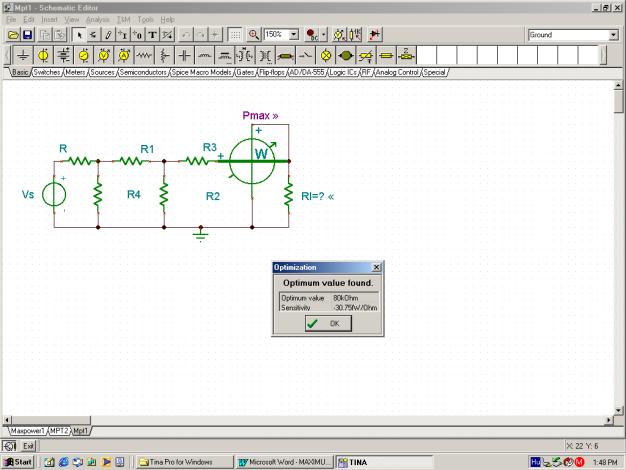
After Optimization, the value of RI is automatically updated to the value found. If we next run an interactive DC analysis by pressing the DC button, the maximum power is displayed as shown in the following figure.

NORTON’S THEOREM

SUPERPOSITION THEOREM