THREE PHASE NETWORKS

Click or Tap the Example circuits below to invoke TINACloud and select the Interactive DC mode to Analyze them Online.
Get a low cost access to TINACloud to edit the examples or create your own circuits

MAXIMUM POWER TRANSFER IN AC CIRCUITS

OHM’S LAW

The alternating current networks that we have studied so far are widely used to model AC mains electric power networks in homes. However, for industrial use and also for electric power generation, a network of AC generators is more effective. This is realized by polyphase networks consisting of a number of identical sinusoidal generators with a phase angle difference. The most common polyphase networks are two- or three-phase networks. We will limit our discussion here to three-phase networks.

Note that TINA provides special tools for drawing three-phase networks in the Special component toolbar, under the Stars and Y buttons.

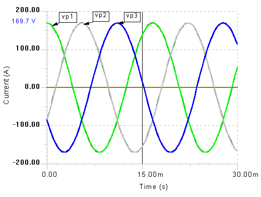
A three-phase network can be seen as a special connection of three single phase or simple AC circuits. Three-phase networks consist of three simple networks, each having the same amplitude and frequency, and a 120° phase difference between adjacent networks. The time diagram of the voltages in a 120V_eff system is shown in the diagram below.

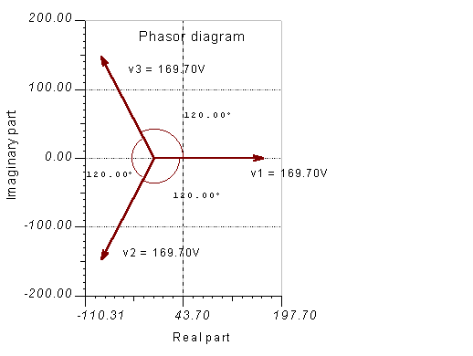
We can also represent these voltages with phasors using TINA’s Phasor Diagram.

Compared to single-phase systems, three phase networks are superior because both the power stations and the transmission lines require thinner conductors for transmitting the same power. Due to the fact that one of the three voltages is always non-zero, three-phase equipment has better characteristics, and three-phase motors are self-starting without any additional circuitry. It is also much easier to convert three-phase voltages into DC (rectification), due to the reduced fluctuation in the rectified voltage.

The frequency of three-phase electric power networks is 60 Hz in United States and 50 Hz in Europe. The single phase home network is simply one of the voltages from a three-phase network.

In practice, the three phases are connected in one of two ways.

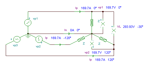
1) The Wye or Y-connection, where the negative terminals of each generator or load are connected to form the neutral terminal. This results in a three-wire system, or if a neutral wire is provided, a four-wire system.

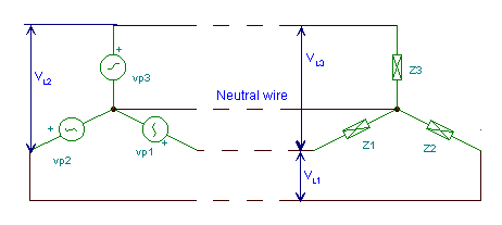
The V_p1,V_p2,V_p3 voltages of the generators are called phase voltages, while the voltages V_L1,V_L2,V_L3 between any two connecting lines (but excluding the neutral wire) are called line voltages. Similarly, the I_p1,I_p2,I_p3 currents of the generators are called phase currents while the currents I_L1,I_L2,I_L3 in the connecting lines (excluding the neutral wire) are called line currents.

In Y-connection, the phase and line currents are obviously the same, but the line voltages are greater than the phase voltages. In the balanced case:

Let ‘s demonstrate this by a phasor diagram:

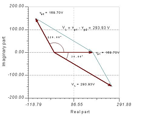
Let’s calculate V_L for the phasor diagram above using the cosine rule of trigonometry:

Now let’s calculate the same quantity using complex peak values:

V_p1 = 169.7 e^{j 0 °} = 169.7

V_p2 = 169.7 e^{j 120 °} = -84.85+j146.96

V_L = V_p2 – V_p1 = -254.55+j146.96 ⁼ 293.9 e ^{j150 °}

The same result with the TINA Interpreter:

Similarly the complex peak values of the line voltages

V_L21 = 293.9 e^{j 150 °} V,
V_L23 = 293.9 e^{j 270 °} V,
V_L13 = 293.9 e^{j 30 °} V.

The complex effective values:

V_L21eff = 207.85 e^{j 150 °} V,
V_L23eff = 207.85 e^{j 270 °} V,
V_L13eff = 207.85 e^{j 30 °} V.

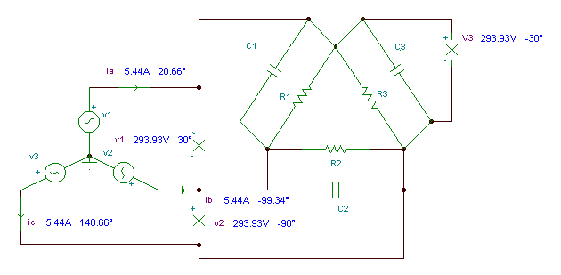
Finally let’s check the same results using TINA for a circuit with

120 V_eff ; V_P1 = V_P2 = V_P3 =169.7 V and Z₁= Z₂ =Z₃ = 1 ohms

2) The delta or D-connection of three phases is achieved by connecting the three loads in series forming a closed loop. This is only used for three-wire systems.

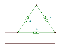
As opposed to a Y-connection, in D -connection the phase and line voltages are obviously the same, but the line currents are greater than the phase currents. In the balanced case:

Let’s demonstrate this with TINA for a network with 120 V_eff Z=10 ohms.

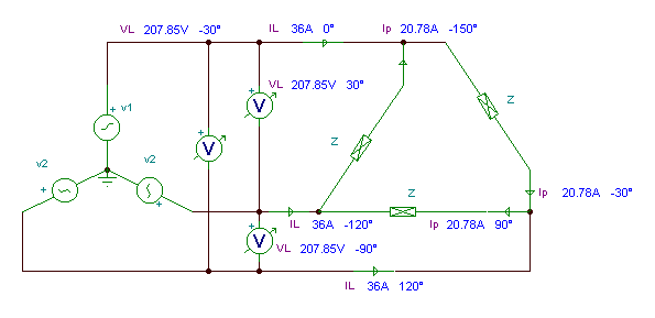
Result: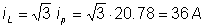

Since either the generator or the load can be connected in D or in Y, there are four possible interconnections: Y-Y, Y- D, D-Y and D- D. If the load impedances of the different phases are equal, the three-phase network is balanced.

Some further important definitions and facts:

The phase difference between the phase voltage or current and the nearest line voltage and current (if they are not the same) is 30 °.

If the load is balanced (i.e. all the loads have the same impedance), each phase’s voltages and currents are equal. Furthermore, in the Y-connection, there is no neutral current even if there is a neutral wire.

If the load is unbalanced, the phase voltages and currents are different Also, in the Y–Y-connection with no neutral wire, the common nodes (star points) are not at the same potential. In this case we can solve for node potential V₀ (the common node of the loads) using a node equation. Calculating V₀ allows you to solve for the phase voltages of the load, current in the neutral wire, etc. Y-connected generators always incorporate a neutral wire.

The power in a balanced three phase system is P_T = 3 V_pI_p cos J = V_LI_L cos J

where J is the phase angle between the voltage and the current of the load.

The total apparent power in a balanced three phase system: S_T = V_LI_L

The total reactive power in a balanced three phase system: Q_T = V_L I_L sin J

Example 1

The rms value of the phase voltages of a three-phase balanced Y-connected generator is 220 V; its frequency is 50 Hz.

a/ Find the time function of the phase currents of the load!

b/ Calculate all the average and reactive powers of the load!

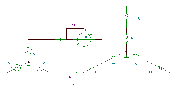
Both the generator and the load are balanced, so we need to calculate only one phase and can get the other voltages or currents by changing the phase angles. In the schematic above we did not draw the neutral wire, but instead assigned ‘earth’ at both sides. This can serve as a neutral wire; however, because the circuit is balanced the neutral wire is not needed.

The load is connected in Y, so the phase currents are equal to the line currents: the peak values:

I_P1 = V_P/(R+j w L) = 311/(100+j314*0.3) = 311/(100+j94.2) = 1.65-j1.55 = 2.26 e^{-j43.3 °} A

V_P1 = 311 V

I_P2 = I_P1 e ^{j 120 °} =2.26 e^{j76.7 °} A

I_P3 = I_P2 e ^{j 120 °} =2.26 e^{-j163.3 °} A

i_P1 = 2.26 cos ( w×t – 44.3 ° ) A

i_P2 = 2.26 cos ( w× t + 76.7 °) A

The powers are also equal: P₁ = P₂ = P₃ = = 2.26²*100/2 = 256.1 W

This is the same as calculated results by hand and TINA’s Interpreter.

Example 2

A three-phase balanced Y-connected generator is loaded by a delta-connected three-pole load with equal impedances. f=50 Hz.

Find the time functions of a/ the phase voltages of the load,

b/ the phase currents of the load,

c/ the line currents!

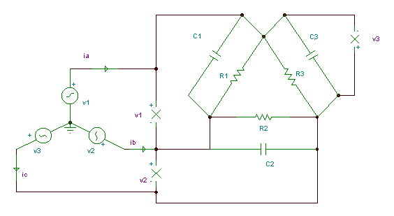
The phase voltage of the load equals the line voltage of the generator:

V_L =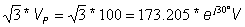

The phase currents of the load: I₁ = V_L/R₁+V_Lj w C = 1.228 + j1.337 = 1.815 e^{j 47.46 °} A

I₂ = I₁ * e^{-j120 °} = 1.815 e^{-j72.54 °} A = 0.543 – j1.73 A

I₃ = I₁ * e^{j120 °} = 1.815 e^{j167.46 °} = -1.772 + j0.394

Seeing the directions: I_a = I₁ – I₃ = 3+j0.933 A = 3.14 e^{j17.26 °} A.

According to the results calculated by hand and TINA’s Interpreter.

Finally an example with an unbalanced load:

Example 3

The rms value of the phase voltages of a three-phase balanced

Y-connected generator is 220 V; its frequency is 50 Hz.

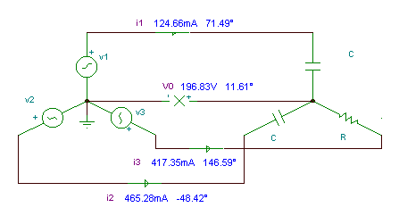
a/ Find the phasor of the voltage V₀ !

b/ Find the amplitudes and initial phase angles of the phase currents !

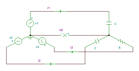
Now the load is an asymmetrical one and we have no neutral wire, so we can expect a potential difference between the neutral points. Use an equation for the node potential V₀:

hence V₀ = 192.71+ j39.54 V = 196.7 e^{j11.6 °} V

and: I₁ = (V₁-V₀)*j w C = 0.125 e^{j71.5 °} A; I₂ = (V₂-V₀)*j w C = 0.465 e^{-j48.43 °}

and I₃ =(V₃-V₀)/R = 0.417 e^{j 146.6 °} A

v₀(t) = 196.7 cos ( w× t + 11.6 ° ) V;

i₁(t) = 0.125 cos ( w× t + 71.5 ° ) A;

i₂(t) = 0.465 cos ( w× t – 48.4 ° ) A;

And, finally, the results calculated by TINA agree with the results calculated by the other techniques.

MAXIMUM POWER TRANSFER IN AC CIRCUITS

OHM’S LAW