 Click or Tap the Example circuits below to invoke TINACloud and select the Interactive DC mode to Analyze them Online.
 Get a low cost access to TINACloud to edit the examples or create your own circuits
As we saw in the previous chapter, impedance and admittance can be manipulated using the same rules as are used for DC circuits. In this chapter we will demonstrate these rules by calculating total or equivalent impedance for series, parallel and series-parallel AC circuits.
Example 1
Find the equivalent impedance of the following circuit:
R = 12 ohm, L = 10 mH, f = 159 Hz
The elements are in series, so we realise that their complex impedances should be added:
Zeq = ZR + ZL = R + j w L = 12 + j*2*p*159*0.01 = (12 + j 9.99) ohm = 15.6 ej39.8° ohm.
Yeq = 1/Zeq = 0.064 e– j 39.8° S = 0.0492 – j 0.0409 S
We can illustrate this result using impedance meters and the Phasor Diagram in
TINA v6. Since TINA’s impedance meter is an active device and we are going to use two of them, we must arrange the circuit so that the meters don’t influence each other.
We have created another circuit just for the measurement of the part impedances. In this circuit, the two meters do not “see” each other’s impedance.
The Analysis/AC Analysis/Phasor diagram command will draw the three phasors on one diagram. We used the Auto Label command to add the values and the Line command of the Diagram Editor to add the dashed auxiliary lines for the parallelogram rule.
The circuit for measuring the impedances of the parts
Phasor diagram showing the construction of Zeq with the parallelogram rule
As the diagram shows, the total impedance, Zeq, can be considered as a complex resultant vector derived using the parallelogram rule from the complex impedances ZR and ZL .
Example 2
Find the equivalent impedance and admittance of this parallel circuit:
R =20 ohm, C = 5 mF, f = 20 kHz
The admittance:

The impedance using the Ztot= Z1 Z2 / (Z1 + Z2 ) formula for parallel impedances:
 Another way TINA can solve this problem is with its Interpreter:
om:=2*pi*20000;
Z:=Replus(R,(1/j/om/C))
Z=[125.8545m-1.5815*j]
Y:=1/R+j*om*C;
Y=[50m+628.3185m*j]
import math as m
import cmath as c
#First define replus using lambda:
Replus= lambda R1, R2 : R1*R2/(R1+R2)
#Lets simplify the print of complex
#numbers for greater transparency:
cp= lambda Z : “{:.4f}”.format(Z)
om=2*c.pi*20000
Z=Replus(R,1/complex(0,1/om/C))
print(“Z=”,cp(Z))
Y=complex(1/R,om*C)
print(“Y=”,cp(Y))
Example 3
Find the equivalent impedance of this parallel circuit. It uses the same elements as in Example 1:
R = 12 ohm and L = 10 mH, at f = 159 Hz frequency.
For parallel circuits, it’s often easier to calculate the admittance first:
Yeq = YR + YL = 1/R + 1/ (j*2*p*f*L) = 1/12 – j /10 = 0.0833 – j 0.1 = 0.13 e–j 50° S
Zeq = 1 / Yeq = 7.68 e j 50° ohm.
Another way TINA can solve this problem is with its Interpreter:
f:=159;
om:=2*pi*f;
Zeq:=replus(R,j*om*L);
Zeq=[4.9124+5.9006*j]
import math as m
import cmath as c
#First define replus using lambda:
Replus= lambda R1, R2 : R1*R2/(R1+R2)
#Lets simplify the print of complex
#numbers for greater transparency:
cp= lambda Z : “{:.4f}”.format(Z)
f=159
om=2*c.pi*f
Zeq=Replus(R,complex(1j*om*L))
print(“Zeq=”,cp(Zeq))
Example 4
Find the impedance of a series circuit with R = 10 ohm, C = 4 mF, and L = 0.3 mH, at an angular frequency w = 50 krad/s (f = w / 2p = 7.957 kHz ).
Z = R + j w L – j / wC = 10 + j 5*104 * 3*10-4 – j / (5*104 *4 * 10-6 ) = 10 + j 15 – j 5
|
Z = (10 + j 10) ohm = 14.14 ej 45° ohms.
The circuit for measuring the impedances of the parts
The phasor diagram as generated by TINA
Starting with the phasor diagram above, let’s use the triangle or geometric construction rule to find the equivalent impedance. We start by moving the tail of ZR to the tip of ZL. Then we move the tail of ZC to the tip of ZR. Now the resultant Zeq will exactly close the polygon starting from the tail of the first ZR phasor and ending at the tip of ZC.
The phasor diagram showing the geometric construction of Zeq
om:=50k;
ZR:=R;
ZL:=om*L;
ZC:=1/om/C;
Z:=ZR+j*ZL-j*ZC;
Z=[10+10*j]
abs(Z)=[14.1421]
radtodeg(arc(Z))=[45]
{other way}
Zeq:=R+j*om*L+1/j/om/C;
Zeq=[10+10*j]
Abs(Zeq)=[14.1421]
fi:=arc(Z)*180/pi;
fi=[45]
import math as m
import cmath as c
#Lets simplify the print of complex
#numbers for greater transparency:
cp= lambda Z : “{:.4f}”.format(Z)
om=50000
ZR=R
ZL=om*L
ZC=1/om/C
Z=ZR+1j*ZL-1j*ZC
print(“Z=”,cp(Z))
print(“abs(Z)= %.4f”%abs(Z))
print(“degrees(arc(Z))= %.4f”%m.degrees(c.phase(Z)))
#other way
Zeq=R+1j*om*L+1/1j/om/C
print(“Zeq=”,cp(Zeq))
print(“abs(Zeq)= %.4f”%abs(Zeq))
fi=c.phase(Z)*180/c.pi
print(“fi=”,cp(fi))
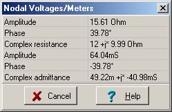
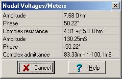
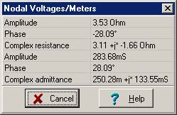
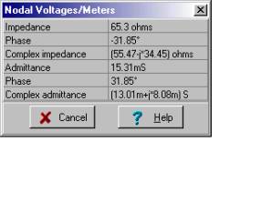
Check your calculations using TINA’s Analysis menu Calculate nodal voltages. When you click on the Impedance meter, TINA presents both the impedance and admittance, and gives the results in algebraic and exponential forms.

Since the circuit’s impedance has a positive phase like an inductor, we can call it an inductive circuit–at least at this frequency!
Example 5
Find a simpler series network that could replace the series circuit of example 4 (at the given frequency).
We noted in Example 4 that the network is inductive, so we can replace it by a 4 ohm resistor and a 10 ohm inductive reactance in series:
XL = 10 = w*L = 50*103 L
® L = 0.2 mH
|
Don’t forget that, since inductive reactance depends upon frequency, this equivalence is valid only for one frequency.
Example 6
Find the impedance of three components connected in parallel: R = 4 ohm, C = 4 mF, and L = 0.3 mH, at an angular frequency w = 50 krad/s (f = w / 2p = 7.947 kHz).
|
Noting that this is a parallel circuit, we solve first for the admittance:
1/Z = 1/R +1/ j w L + jwC = 0.25 – j/15 +j0.2 = 0.25 +j 0.1333
Z = 1/(0.25 + j 0.133) = (0.25 – j 0.133)/0.0802 = 3.11 – j 1.65 =3.5238 e–j 28.1° ohms.
om:=50k;
ZR:=R;
ZL:=om*L;
ZC:=1/om/C;
Z:=1/(1/R+1/j/ZL-1/j/ZC);
Z=[3.1142-1.6609*j]
abs(Z)=[3.5294]
fi:=radtodeg(arc(Z));
fi=[-28.0725]
import math as m
import cmath as c
#Lets simplify the print of complex
#numbers for greater transparency:
cp= lambda Z : “{:.4f}”.format(Z)
#Define replus using lambda:
Replus= lambda R1, R2 : R1*R2/(R1+R2)
om=50000
ZR=R
ZL=om*L
ZC=1/om/C
Z=1/(1/R+1/1j/ZL-1/1j/ZC)
print(“Z=”,cp(Z))
print(“abs(Z)= %.4f”%abs(Z))
fi=m.degrees(c.phase(Z))
print(“fi= %.4f”%fi)
#another way
Zeq=Replus(R,Replus(1j*om*L,1/1j/om/C))
print(“Zeq=”,cp(Zeq))
print(“abs(Zeq)= %.4f”%abs(Zeq))
print(“degrees(arc(Zeq))= %.4f”%m.degrees(c.phase(Zeq)))
The Interpreter calculates phase in radians. If you want phase in degrees, you can convert from radians to degrees by multiplying by 180 and dividing by p. In this last example, you see a simpler way—use the Interpreter’s built in function, radtodeg. There is an inverse function as well, degtorad. Note that this network’s impedance has a negative phase like a capacitor, so we say that—at this frequency—it is a capacitive circuit.
In Example 4 we placed three passive components in series, while in this example we placed the same three elements in parallel. Comparing the equivalent impedances calculated at the same frequency, reveals that they are totally different, even their inductive or capacitive character.
Example 7
Find a simple series network that could replace the parallel circuit of example 6 (at the given frequency).
This network is capacitive because of the negative phase, so we try to replace it with a series connection of a resistor and a capacitor:
Zeq = (3.11 – j 1.66) ohm = Re –j / wCe
Re = 3.11 ohm w*C = 1/1.66 = 0.6024
hence
Re = 3.11 ohm
C = 12.048 mF
You could, of course, replace the parallel circuit with a simpler parallel circuit in both examples
Example 8
Find the equivalent impedance of the following more complicated circuit at frequency f=50 Hz:
om:=2*pi*50;
Z1:=R3+j*om*L3;
Z2:=replus(R2,1/j/om/C);
Zeq:=R1+Replus(Z1,Z2);
Zeq=[55.469-34.4532*j]
abs(Zeq)=[65.2981]
radtodeg(arc(Zeq))=[-31.8455]
import math as m
import cmath as c
#Lets simplify the print of complex
#numbers for greater transparency:
cp= lambda Z : “{:.4f}”.format(Z)
#Define replus using lambda:
Replus= lambda R1, R2 : R1*R2/(R1+R2)
om=2*c.pi*50
Z1=R3+1j*om*L3
Z2=Replus(R2,1/1j/om/C)
Zeq=R1+Replus(Z1,Z2)
print(“Zeq=”,cp(Zeq))
print(“abs(Zeq)= %.4f”%abs(Zeq))
print(“degrees(arc(Zeq))= %.4f”%m.degrees(c.phase(Zeq)))
We need a strategy before we begin. First we’ll reduce C and R2 to an equivalent impedance, ZRC. Then, seeing that ZRC is in parallel with the series-connected L3 and R3, we’ll compute the equivalent impedance of their parallel connection, Z2. Finally, we calculate Zeq as the sum of Z1 and Z2.
Here’s the calculation of ZRC:

Here’s the calculation of Z2:

And finally:
Zeq = Z1 + Z2 = (55.47 – j 34.45) ohm = 65.3 e–j31.8° ohm
according to TINA’s result.